There is no allowed spherical harmonic with $m=l+1$, so $L_{+}{Y}_l^l=0$. The equation $-i\hslash {\partial }_{\varphi }Y=\hslash lY$ first gives $Y=f(\theta )e^{il\varphi }$. Combining the differential expressions for $L_x,L_y$ yieldsIts annihilation of the highest-weight state becomesIntegrating $f^{\prime }/f=l\cot \theta$ gives $f=C{\sin }^l\theta$, with the constant solution included for $l=0$. HenceThe phase $e^{il\varphi }$ is single valued for integral orbital quantum number $l$; normalization fixes only $|C|$, leaving a conventional constant phase.

The spherical harmonics satisfyCommuting $L^2$ or $L_z$ past $L_{\pm }$ therefore givesFor a nonzero result these are the eigenvalue equations with unchanged $l$ and shifted magnetic quantum number. Taking the squared norm, using $L_{\mp }{L}_{\pm }=L^2-L_z^2\mp \hslash L_z$, fixes the conventional coefficient:At the appropriate endpoint the coefficient is zero. The zero vector is not itself an eigenstate.

Hermiticity of the Cartesian angular momentum components givesThe angular momentum commutation relations $[L_i,L_j]=i\hslash {ϵ}_{ijk}{L}_k$ implyFor example, $[L_z,L_x+i{L}_y]=i\hslash L_y+\hslash L_x=\hslash L_{+}$. The two terms in $[L_x^2+L_y^2+L_z^2,L_i]$ cancel in pairs, giving the first commutator. Also $[L_{+},L_{-}]=2\hslash L_z$.

For a conditional spin measurement of identical fermions addressing the $z$ component in one spatial mode, the Born rule givesConditioned on this result, the mode spin state is $|{\uparrow }_a{\downarrow }_b⟩$; the other outcome produces $|{\downarrow }_a{\uparrow }_b⟩$. The spin product is not a spin-exchange eigenstate. The measurement has selected an addressed mode and recorded an outcome, so this conditional spin description distinguishes the measured subsystem.

The full electron wavefunction still obeys fermionic exchange symmetry. For example, the conditional spin-up outcome in spatial mode $a$ is represented in particle coordinates byIt is antisymmetric under full particle exchange. Thus the loss of a definite symmetry of the conditional spin product does not mean that measurement turns identical electrons into distinguishable particles. If the outcome is discarded, the mode spin state is instead the equal mixture of the two opposite-spin products. The measurement must specify which spatial mode is addressed for the conditional statement to be operationally meaningful.

Write $\Psi =(|\downarrow \uparrow ⟩+|\uparrow \downarrow ⟩)/\sqrt{2}$. Each term has cancelling $z$ components, so $S_z\Psi =0$. In the formula for $S^2$, the first three terms contribute $(3/2-1/2){\hslash }^2\Psi ={\hslash }^2\Psi$. The two ladder products exchange the two terms and contribute another ${\hslash }^2\Psi$. ThereforeThis spin state is symmetric; the accompanying spatial state must be antisymmetric for two electrons. A labelled product $|{\downarrow }_1{\uparrow }_2⟩$ alone is not an eigenstate of spin exchange: its exchanged vector is orthogonal to it. Thus it cannot supply a definite exchange symmetry when multiplied by a fixed symmetric spatial factor.

This does not prohibit opposite spins in different spatial orbitals. For example, with orthonormal orbitals ${\varphi }_a,{\varphi }_b$, the Slater determinantis a valid antisymmetric two-electron state. What fails is treating persistent particle labels as physically distinguishable identities without the required antisymmetrization.

Expanding the total angular momentum and replacing transverse components by ladder operators givesThe particle exchange operator obeys $P_{12}^2=I$ and $P_{12}{s}_{1\alpha }{P}_{12}=s_{2\alpha }$, with the reverse relation for index $2$. These statements also apply to the ladder operators. Exchanging the indices preserves $s_1^2+s_2^2$ and $s_{1z}+s_{2z}$; it interchanges the last two terms in $S^2$. Operators on different tensor factors commute. HenceThe full particle exchange includes the spin coordinates as well as the spatial coordinates.

The spin Hilbert space is a tensor product of two two-dimensional spaces and therefore has dimension four. Angular momentum addition decomposes it asThese are three orthogonal triplet states and one singlet state. For identical electrons the complete wavefunction must also satisfy fermionic exchange symmetry: a symmetric triplet spin factor accompanies an antisymmetric spatial factor, whereas the antisymmetric singlet spin factor accompanies a symmetric spatial factor. If both electrons occupy the same spatial orbital, only the singlet spin factor is allowed. The four-dimensional spin space does not assert four allowed spin states for that particular spatial occupation.

Suppress the fixed individual quantum numbers $s_1=s_2=1/2$. In the coupled basis, ordered on both rows and columns as $|1,1⟩,|1,0⟩,|1,-1⟩,|0,0⟩$, the total-spin eigenvalues giveHere the first three entries form the triplet state sector and the last is the singlet state. For the product basis, useThe first term has diagonal entries ${\hslash }^2(1,-1,-1,1)/4$. Each nonzero exchange term flips $|\uparrow \downarrow ⟩$ to $|\downarrow \uparrow ⟩$ or back, with coefficient ${\hslash }^2/2$. With rows and columns ordered as $|\uparrow \uparrow ⟩,|\uparrow \downarrow ⟩,|\downarrow \uparrow ⟩,|\downarrow \downarrow ⟩$,The change of basis is made explicit by $|1,0⟩=(|\uparrow \downarrow ⟩+|\downarrow \uparrow ⟩)/\sqrt{2}$ and $|0,0⟩=(|\uparrow \downarrow ⟩-|\downarrow \uparrow ⟩)/\sqrt{2}$, with $|1,\pm 1⟩=|\uparrow \uparrow ⟩,|\downarrow \downarrow ⟩$. The resulting eigenvalues reproduce the diagonal coupled matrix.

For two spin one-half particles, $s_1^2=s_2^2=3{\hslash }^2/4$. Squaring $\mathbf{S}={\mathbf{s}}_1+{\mathbf{s}}_2$ givesTake $a,b$ real so that $f$ is Hermitian. Since $[S^2,S_z]=0$, the displayed polynomial implies $[f,S^2]=[f,S_z]=0$. There is a common orthonormal eigenbasis, so all three observables can be simultaneously certain in a common eigenstate. Commutation does not mean that every quantum superposition has definite values of all three.

Differentiate ${\dot{c}}_2=-i\gamma e^{2i\Omega t}{c}_1$ and substitute the equation for ${\dot{c}}_1$. The result isPutting $c_2=e^{i\Omega t}u$ removes the first derivative and gives $\ddot{u}+{\kappa }^{2}u=0$, where $\kappa =\sqrt{{\Omega }^2+{\gamma }^2}$. For $\kappa >0$ the general solution isThe initial spinor fixes $c_1(0)=1,c_2(0)=0$, and the first-order coupled equation fixes the second initial datum ${\dot{c}}_2(0)=-i\gamma$. Thus $A=0$, $B=-i\gamma /\kappa$, andTheir squared magnitudes sum to one. If both $\Omega$ and $\gamma$ vanish, the initial amplitudes simply remain $(1,0)$; the formulas have that continuous limit.

Source convention correction. For positive $\gamma$, the printed expression for $c_2$ lacks the factor $-i$ required by the stated basis and initial vector. A concrete test is its derivative at $t=0$: the printed expression gives $+\gamma$, whereas the Schrödinger equation gives $-i\gamma$. Multiplying only $c_2$ by a phase changes the relative quantum phase. One may change the overall phase of the entire spinor, but must then transform $c_1$ and its initial amplitude as well. The printed modulus nevertheless gives the correct transition probability.

Insert the expansion with amplitudes $c_1,c_2$ and the two unperturbed dynamical phases into $i\hslash \dot{\Psi }=(H_0+V)\Psi$. Differentiation of the explicit phases cancels $H_0$, leavingEquivalently, with $\Omega =(\omega -{\omega }_0)/2$,These interaction-picture equations conserve $|c_1{|}^2+|c_2{|}^2$. They are exact for the circularly rotating magnetic drive; a rotating-wave approximation has not been used.

In the ordered basis $|+⟩,|-⟩$, the transverse magnetic field producesThe off-diagonal complex exponentials follow directly from $\cos \omega t\mp i\sin \omega t$. This matrix is Hermitian at every time.

With $\mathbf{B}=B_0\hat{\mathbf{z}}$ and $S_z=(\hslash /2){\sigma }_z$,ThusFor $B_0>0$, spin down is the lower energy eigenstate. The negative electron magnetic moment is already accounted for in the positive coefficient multiplying $\mathbf{S}\cdot \mathbf{B}$ in the given Hamiltonian.

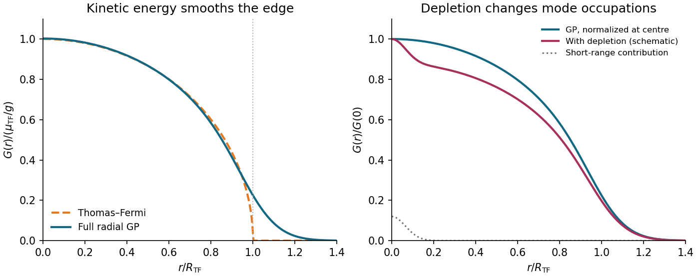
The Hartree product state underlying the Gross–Pitaevskii equation has the factorized one-body coherence of a Hartree condensate. Choosing its nodeless ground state orbital real givesIn particular, the Thomas–Fermi approximation for a condensate from part (d) predictsThe curve starts at $\mu /g$, decreases with zero slope at the origin, and reaches zero with an infinite slope at $R$. Restoring the kinetic energy in the full Gross–Pitaevskii equation rounds that edge and produces a nonzero tail. This corrects the Thomas–Fermi approximation for a condensate, but the resulting one-body density matrix still factorizes.

The additional missing physics is quantum depletion. Interactions scatter pairs of bosons into orbitals outside the Bose-Einstein condensate even at zero temperature. In terms of the true Bose-Einstein condensate orbital ${\phi }_0$ the exact one-body density matrix decomposes asThe single-orbital Hartree product state sets $N_0=N$ and omits ${\rho }_{\mathrm{ex}}$ altogether. In a weakly interacting Bose gas, Bogoliubov theory adds a comparatively short-range noncondensed contribution near the origin, together with reduced weight in the broad Bose-Einstein condensate component. The central value remains the total number density, not just the condensate density. Its numerical shift relative to the original Gross–Pitaevskii equation solution also depends on the interaction-induced redistribution of number density; it is not fixed by the condensate fraction alone.

In the large-$N$ Gross–Pitaevskii equation, dropping the kinetic energy gives $[\kappa r^2/2+gn(r)-\mu ]\Psi (r)=0$. The physical nonnegative Thomas–Fermi approximation for a condensate is thereforewhere $(z{)}_{+}=\max (z,0)$ and $R$ is the cloud radius. Its particle number isThus the two-dimensional Thomas–Fermi condensate obeysHere $N=\int n{d}^{2}r$ is a total particle number. Keeping the exact pair count in the fixed-$N$ Hartree product state would replace $g$ by $g(1-1/N)$ in these formulas expressed in terms of $n=N|\varphi {|}^2$.

The approximation is best at the centre, $r=0$, and worst near the edge, $r=R$. For example its omitted quantum pressure of a condensate, evaluated on the interior profile, isIt is smallest at the centre and diverges at the artificial sharp edge. The central healing length ${\xi }_0=\hslash /\sqrt{2m\mu }$ is much smaller than $R$ when $\mu \gg \hslash \omega$, since $R/{\xi }_0=2\mu /(\hslash \omega )$. This is the bulk validity condition; the full Gross–Pitaevskii equation smooths the edge and gives a decaying tail outside $R$.

For a normalized orbital $\int d^{2}r|\varphi {|}^2=1$, the symmetric Hartree product state and its equivalent Fock space form areThere are exactly $N(N-1)/2$ interacting pairs, so the expectation value of the grand Hamiltonian is the functionalAt fixed $N$ the term $-\mu N$ is constant. Enforce wavefunction normalization separately by varying ${\mathcal{E}}_{\mu }-N\eta (\int |\varphi {|}^2-1)$ with respect to ${\varphi }^{\ast }$. The resulting stationary Gross–Pitaevskii equation for the normalized orbital isThe Lagrange multiplier $\eta$ enforces the norm; fixed-$N$ variation cannot identify it with the independently inserted chemical potential merely by differentiating the constant $-\mu N$.

For the standard large-$N$ convention put $\Psi =\sqrt{N}\varphi$, so $n=|\Psi {|}^2$ and $\int n=N$, and replace $N-1$ by $N$. Varying the resulting grand energy functionalwith unrestricted $\Psi$ givesEquivalently, at fixed $N$ this same $\mu$ is chosen as the normalization Lagrange multiplier. This is the chemical potential convention used below. The contact interaction coupling $g$ has dimensions of energy times area in two dimensions.

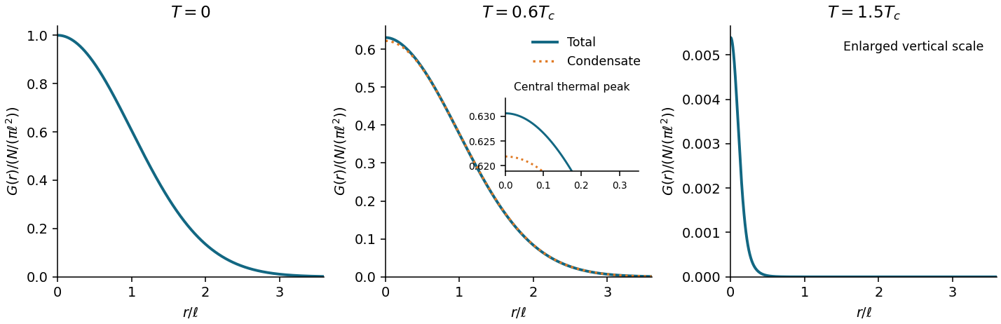
Write $G(r)=⟨{\psi }^{†}(0)\psi (\mathbf{r})⟩$, $r=|\mathbf{r}|$, and ${\ell }^2=\hslash /(m\omega )$. At zero temperature all $N$ particles occupy ${\varphi }_0(\mathbf{r})=(\ell \sqrt{\pi }{)}^{-1}{e}^{-r^2/(2{\ell }^2)}$. Expanding the bosonic annihilation operator in single-particle orbitals givesThis one-body density matrix is a Gaussian function of width $\ell$; it contains one wavefunction evaluated at $r$, so its exponent is half that of the spatial number density $N|{\varphi }_0(r){|}^2$. In particular,the total number density at the trap centre, including condensed and noncondensed particles.

At positive temperature, with occupations ${\overline{n}}_a$ of the trap energy eigenstates, the exact ideal-gas decomposition isFor $\hslash \omega \ll k_{B}T<k_B{T}_c$, the sketch has a broad Bose-Einstein condensate component on scale $\ell$ and a narrower thermal peak near the origin. On approaching $T_c$ the broad component loses its weight $N_0$, while the thermal part remains. Above $T_c$ there is no macroscopic broad Bose-Einstein condensate component; close to $T_c$, low energy levels can still give a shoulder, so a single narrow Gaussian function is only a high-temperature description. At $k_{B}T\lesssim \hslash \omega$ individual excited energy levels matter and the two-scale description need not apply.

For $T\gg T_c$ the Maxwell-Boltzmann distribution applies. The leading off-diagonal one-body density matrix isHere ${\sigma }_r$ is the Gaussian function width defined by $e^{-r^2/(2{\sigma }_r^2)}$, and ${\lambda }_T$ is the thermal de Broglie wavelength. The thermal cloud itself extends over the much larger spatial scale $\sqrt{k_{B}T/\kappa }$; this is a correlation width, not the cloud radius.

Measure single-particle energy from the quantum harmonic oscillator ground state energy $\hslash \omega$, and write $\tilde{\mu }={\mu }_{\mathrm{physical}}-\hslash \omega \le 0$. The Bose-Einstein distribution and the supplied density of states giveThis excited-state population increases with the chemical potential and has the finite saturation valueAny additional particles must occupy the ground state: this is two-dimensional harmonic-trap Bose condensation. The critical temperature and the condensate fraction are thereforeHere $N$ is the total particle number, the integral of the inhomogeneous number density over the trap; there is no fixed uniform area in which $N$ itself is a number density. Equivalently $N\kappa ={\pi }^{2}m(k_B{T}_c{)}^2/(6{\hslash }^2)$ relates the trap population to the critical temperature. Harmonic confinement changes the low-energy density of states and permits this saturation in two spatial dimensions.

These formulas are leading large-$N$ results with $k_B{T}_c\gg \hslash \omega$. A sharp transition belongs to the trapped-gas thermodynamic limit $N\to \infty$, $\omega \to 0$ at fixed $N{\omega }^2$; a finite trap has finite-size rounding. In particular, finite $N_0$ requires $\tilde{\mu }=-k_{B}T\log (1+1/N_0)<0$, approaching zero in the condensation limit.