Topics (384k) Articles (398k) Users (410) Discussions (242) Comments (383) Files (13k) New article

Regurgitant volume is the amount of blood transported backward through a leaking heart valve over a specified interval, usually a cardiac cycle. In mitral regurgitation, it is backward transport from the left ventricle towards the left atrium during ventricular systole. It measures an integrated volume rather than a peak velocity or one still image of the jet.
For a fixed measurement surface with normal pointing in the backward direction, the instantaneous backward flux is the surface integral of the corresponding positive normal velocity. Integrating over time givesA moving surface instead requires velocity relative to that surface. This convention separates material transported through a boundary from the motion of the boundary itself.
An imaging estimator combines an effective regurgitant orifice area with a velocity-time integral. If the effective area is approximately constant over the interval,The technical recommendations describe this area-times-integrated-velocity approach and complementary volumetric methods.[ref]
For stipulated and VTI 150 cm, the estimate is mL. Equal peak velocities do not ensure equal VTI: two triangular velocity pulses of height 5 m/s and durations 0.10 and 0.20 s have integrals 25 and 50 cm. At the same effective area, their modeled backward volumes are 5 and 10 mL. These are illustrative pulses, not observed valve measurements.
A changing effective area cannot generally be pulled out of the time integral. A peak-area measurement multiplied by the full VTI can therefore answer a different question from integrating the changing area and velocity together. Independently, the ventricular balance requires compatible total and forward stroke volumes. The regurgitant fraction then divides by the relevant total volume; it does not replace the underlying amount measurement.
The regurgitant fraction is the proportion of a valve-related total ejected blood volume that returns through the leaking valve. For the left ventricular balance used to assess mitral regurgitation, let be total ventricular stroke volume, the matched forward aortic volume and the regurgitant volume. With no other abnormal communication or confounding valve leak,The imaging recommendations use complementary volume and flow measurements to quantify these quantities.[ref]
Recommendations for Noninvasive Evaluation of Native Valvular Regurgitation by William A. Zoghbi and others. Section II.B.6, volumetric methods; Figure 8, p.316
An original example takes mL and mL. Then mL and RF is 30%. The quotient instead expresses leakage relative to forward delivery; it is not the same fraction. The denominator is part of the definition.
Equal fractions also need not indicate equal transported amounts. A 30 mL leak out of 100 mL and a 60 mL leak out of 200 mL both have RF 30%. Conversely, an unchanged 30 mL regurgitant volume gives RF 50% if total ejection falls to 60 mL. These stipulated cases isolate the normalization rather than assigning a clinical severity category.
The two measurements in a derived RF may share errors. For , first-order propagation givesThe covariance term should follow the actual acquisition and data reduction, rather than assuming independence because forward and total volume have different names.[ref]
Mitral annular excursion is displacement of the mitral annulus over a specified part of the cardiac cycle. A commonly used longitudinal observation follows an annular landmark along the cardiac long axis during ventricular systole. The reference position, direction and endpoints are part of the measurement; displacement is distinct from annular area or leaflet coaptation.
The measurement question can be written explicitly. For a fixed unit axis and landmark position , defineAn original 10 mm displacement viewed along an axis tilted by projects to mm. Thus changing the observation direction changes the reported excursion even for the same motion. A single landmark also need not represent every part of a deforming mitral annulus.
A primary human study used cine magnetic resonance imaging, measuring longitudinal displacement in long-axis views and stroke volume in short-axis views. Its model combined displacement with a ventricular short-axis area.[ref]
Atrioventricular plane displacement is the major contributor to left ventricular pumping in healthy adults, athletes, and patients with dilated cardiomyopathy by Marcus Carlsson and others. Abstract, Methods
In an original rigid-piston approximation, area moving axially by sweeps volume . Areas 20 and 40 cm paired with displacements 1 and 0.5 cm both give 20 mL. Smaller excursion need not imply a smaller geometric swept volume when area differs; this model area is not automatically the mitral opening area.A complementary experiment by C. Carlhäll and colleagues implanted markers around the mitral annulus and ventricular wall in six sheep. Biplane fluoroscopy reconstructed three-dimensional marker motion, and tetrahedron-based estimates assessed annular contributions to filling while loading and contraction were varied.[ref]
Contribution of mitral annular dynamics to LV diastolic filling with alteration in preload and inotropic state by C. Carlhäll and others. Abstract, experimental methods
This connects a displacement measurement to moving-chamber geometry. The changing boundary, surrounding deformation and blood flow must be distinguished when relating mitral annular excursion to filling or ejection.The conditional pulse-energy mean given emission averages over emitted optical pulses rather than all commands or all detected events. If denotes an emission event and energy is zero when no pulse is emitted, the conditional expectation identity givesThe left side is energy per trigger. The conditional mean is energy per emitted pulse. Missing-pulse bias in average-power inference explains the corresponding rate denominator.
For an original distribution, let emission probability be . Conditional on emission, energies and are equally likely. The emitted-pulse mean is , whereas the per-trigger mean is . At nominal triggering, average pulse power is ; the actual emission rate gives the same power when multiplied by .
Now let a perfect threshold receiver detect only energies above . Its detected-event mean is and its event probability per trigger is . This is detection-threshold selection bias in pulse-energy means: the detector conditions on a narrower event than emission. The undetected records include both failed emissions and the weaker emitted pulses.
A calibrated pulse monitor, trigger counter and known detection response help distinguish the denominators. A total-energy measurement alone need not identify the missing weak-pulse distribution. Historical calorimetric inference combines total energy, injection time and pulse rate, so the rate must match the population whose mean is reported.[ref]
An unsplittable free-block remainder is the positive suffix left by a proposed allocation that is too small to retain as a valid independent free list record. Its size is below the allocator's minimum free-block size. The region still contains unused bytes, but the chosen representation cannot manage it as a separate free extent. The issue arises because free-region metadata can occupy the regions themselves.[ref]
Let a chosen block have size , let the proposed allocated extent after header/alignment rounding be , and let the minimum free size be . With remainder , an allocator that absorbs an undersized suffix usesThis is one possible policy, not a mandatory allocator interface. The absorbed suffix adds bytes of internal fragmentation beyond the bookkeeping and rounding already included in .
For an original example, take bytes, an8-byte allocated header,16-byte block granularity and bytes. A56-byte payload gives , leaving a representable32-byte free block. A57-byte payload instead gives , leaving an unusable16-byte suffix. Absorbing it reserves all96 bytes. Increasing the request by just one byte has therefore increased this allocation's occupied extent by32 bytes.
If and all extents are multiples of a granularity , a positive absorbed suffix is at most bytes. Without that granularity condition, the general integer-byte bound is . Choosing another free block or another representation can change the tradeoff. Later memory block coalescing can recover adjacent space when allocations are returned, but it does not make an invalid intermediate free record representable.
For fixed positive integer coefficients and a sequence of positive integers , the Milliken-Taylor system isThe ordered blocks need not be consecutive intervals, but they are disjoint and every index of one block precedes every index of the next. This is a set of values from all allowed block choices, rather than just one weighted sum.
For and , blocks and give . Choosing and gives .
The Milliken–Taylor theorem guarantees that for any finite coloring of the positive integers and fixed positive coefficient vector, some infinite generating sequence makes the entire system monochromatic. The special case is the finite-sums conclusion of Hindman's theorem.[ref]
Polynomial Extensions of the Milliken-Taylor Theorem by Vitaly Bergelson and others. Definition1.5 and Theorem1.6
A compressed coefficient vector is a finite coefficient sequence with no zero entries and no equal consecutive entries. Its compression is obtained by first deleting zeros and then replacing each consecutive run of equal values by one value. For positive vectors, the zero-deletion step is vacuous.
For example, compresses to , and compresses to . Repeated values separated by a genuinely different value remain: is already compressed. Thus compression is a run operation, not replacement by the set of distinct entries.
The notion records coefficient patterns in Milliken-Taylor systems and their separation under finite colorings. It does not assert that replacing a vector by its compression leaves the exact generated set unchanged for a fixed sequence: requires two nonempty ordered index blocks, whereas permits a single block with one index. The canonical pattern and the precise block constraints are different data.[ref]
Separating Milliken-Taylor Systems with Negative Entries by Neil Hindman and others. Definition1.5, compression of coefficient sequences
Nominal section feed is the intended advance of specimen relative to knife between successive cutting strokes of a microtome. It specifies a machine setting or commanded increment. It is distinct from the recovered physical section thickness, which can change through cutting and handling, and from the separation of sections selected for an image stack.
JEOL describes presenting the block to a diamond knife by a preset advance and then making the cutting stroke. It also notes that material hardness and environmental temperature can cause recovered sections to differ from the preset thickness.[ref]
Ultramicrotomy by JEOL. Glossary, preset feed/cutting sequence and following paragraph on actual thickness
Consequently the feed record is useful acquisition metadata but does not independently verify thickness.An original acquisition ledger illustrates a changing feed. Let the ideal block face before cutting be at , and stipulate successive feed commands of . If motion follows each command exactly, successive cutting planes lie atIf images represent the newly exposed faces after cuts 1 and 4, their separation is , not three times the initial setting. This statement concerns block-face positions. For images assigned to centres of collected slabs, the coordinate convention must also account for their thicknesses: in this ideal example, centres of slabs 1 and 4 are and , a separation of , while centres of slabs 2 and 3 are and , separated by rather than their face spacing of .
Retain feed changes, cutting order, omitted images and the coordinate convention used by the image stack axis calibration. Independently measuring specimen advance tests the feed mechanism; measuring recovered physical section thickness tests a different outcome. Backlash or thermal expansion can affect the first, while section compression and other deformation can affect the second. The ideal ledger assumes neither kind of discrepancy.
Microbial cryopreservation preserves viable microorganisms at very low temperature for later recovery. It provides stored starting material for future experiments, reducing repeated propagation and the associated opportunities for contamination or changes in inherited characteristics. Recovery, purity and identity remain separate properties to verify.[ref]
Bacteriology Culture Guide by ATCC. Preservation, reasons for maintaining frozen stocks; Bacterial Authentication
Freezing can injure a cell even though low temperature greatly slows its activity. Formation of ice removes liquid water from the surrounding solution and concentrates its dissolved substances; intracellular ice can damage cellular structures. Water movement by osmosis links the external changes to cellular dehydration. Microbial cryoprotectants, including glycerol, help protect the material, but preservation performance depends on the particular organism and conditions.[ref]
Mycology Culture Guide by ATCC. Preservation: Cryopreservation, Overview and Freeze Medium
A constructed recovery measurement makes the accounting explicit. Suppose equal original-volume equivalents of a benign yeast suspension give colony-forming units before storage and after recovery, using the same assay and correcting for any dilution. The estimated recovery fraction isThese are counts of colony-producing units under the assay conditions. Clumps can form single colonies, so the result does not by itself show that exactly seventy percent of individual cells survived. Nor does a high recovery fraction establish unchanged genotype or every original phenotype.
The point of maintaining a preserved reference is reproducibility: separate experiments can begin from material derived from the same stored stock. Microbial cryopreservation retains frozen material, whereas freeze-drying removes water from frozen material. They are different preservation strategies, whose suitability must be established for the material concerned.[ref]
Bacteriology Culture Guide by ATCC. Preservation, Cryopreservation and Lyophilization
A colony-forming unit, abbreviated CFU, is a unit of viable material that produces a distinguishable colony under specified assay conditions. It may begin as one cell or as a clump. Counting colonies therefore measures colony-producing units, rather than automatically counting every living cell in the original sample.[ref]
Bacteriological Analytical Manual Chapter 3: Aerobic Plate Count by the Food and Drug Administration (January 2026). Recording counts, p.8: chains arising from clumps and distinct sources
A measured concentration also requires an accounting of sample volume and dilution. In a simple plate-count model with colonies, plated volume and dilution fraction , the original-sample estimate isIf is in millilitres, is in CFU per millilitre. The fraction is the amount of original sample in one volume of the diluted preparation; it is not the reciprocal dilution factor.[ref]
Bacteriological Analytical Manual Chapter 3: Aerobic Plate Count by the Food and Drug Administration (January 2026). SectionD, example2.2a, p.7: divide count by original-homogenate volume
For an original benign-yeast example, suppose two matched measurements yield50 and70 colonies, each from at . Pooling the counts and effective volumes givesThis assumes a well-mixed preparation, comparable recovery and distinct countable colonies. It is an arithmetic illustration, not a recommendation for culturing a particular organism.
A culture medium, incubation conditions and recovery state determine which viable units become visible. A zero count in a finite tested volume does not prove that no viable material exists anywhere in the sample. Crowded colonies, clumping and assay inhibition also affect interpretation; the method and its reporting conventions should accompany the result.[ref]
Bacteriological Analytical Manual Chapter 3: Aerobic Plate Count by the Food and Drug Administration (January 2026). Recording counts, p.8: spreaders and plates with no CFU
Methylorubrum extorquens is a species of bacteria and the type species of Methylorubrum. The older combination
Methylobacterium extorquens names the same species: LPSN records it as a homotypic synonym, meaning that the two names share a nomenclatural type.[ref] Experimental results still need a specified bacterial strain; a species name alone does not identify every tested culture.Methylorubrum extorquens AM1 is a model for facultative methylotrophy. Its studied pathway converts methanol to formaldehyde, with carbon subsequently divided between oxidation toward carbon dioxide and carbon assimilation into cellular material.[ref]
A 2005 experiment compared AM1-derived mutants with a reference strain during colonization of Medicago truncatula. Mutants defective in methylotrophy lost ground in competition, yet could reach comparable populations when tested separately. This distinction supports a competitive advantage from methanol use without making it the only usable carbon source.[ref]
Methylotrophic metabolism is advantageous for Methylobacterium extorquens during colonization of Medicago truncatula under competitive conditions by Abdoulaye Sy and others. Abstract and Figures 2–3, competitive versus single-inoculation comparisons
In an illustrative count, a population share changing from to halves the strain's share; it does not show that its absolute number of cells halved. Both the fraction and the total count are needed to distinguish relative success from population decline.Formylmethionine, usually written fMet in bacterial initiation, is methionine whose amino group bears a formyl group, . The nitrogen modification makes an amide; it does not replace the sulfur-containing side chain. The free neutral L-form has molecular formula .[ref]
In canonical bacterial initiation, methionine is first attached to an initiator transfer RNA and then formylated on that carrier. Bacterial initiation factor IF2 recognizes the formylated end during assembly at the ribosomal P site. Free formylmethionine, its tRNA-bound form and the initiating residue in a peptide are different chemical states.[ref]
Large-Scale Movements of IF3 and tRNA during Bacterial Translation Initiation by Tanweer Hussain and others. Introduction, recognition of the formylmethionyl moiety by IF2
An original atom balance clarifies the modification. Replacing one amino-nitrogen hydrogen in free methionine, , by gives a net addition of and hence . The free-compound formula does not include the transfer RNA or account for its ester linkage.
Formylation alone is not a complete initiation signal. In a primary experiment, anticodon-stem variants of an Escherichia coli initiator were purified, aminoacylated and formylated. Some retained IF2 binding but lost efficient P-site binding and initiation. The carrier's RNA structure therefore contributes recognition information beyond its attached formylmethionine.[ref]
Escherichia coli formylmethionine tRNA: mutations in GGGCCC sequence conserved in anticodon stem of initiator tRNAs affect initiation of protein synthesis and conformation of anticodon loop by B. L. Seong and U. L. RajBhandary. Abstract, separate initiation-factor binding, P-site binding and protein-synthesis assays
The root apical meristem is the region near a growing root tip that maintains dividing cells and supplies descendants for root development. It lies behind the root cap and differs from the root elongation zone, where much of the increase in cell length occurs. Producing new cells and enlarging existing cells are related but distinct contributions to growth.[ref]
Cell position can help determine what those descendants become. In a 1995 experiment, selected Arabidopsis thaliana root-meristem cells were removed by laser ablation. The resulting patterns supported positional control of cell fate despite the normally regular relationships among descendants. The authors inferred directional signals from more mature cells toward initial cells.[ref]
Cell fate in the Arabidopsis root meristem determined by directional signalling by C. van den Berg and others. Abstract: ablation, clonal relationships and directional signaling
The experimental contrast is illuminating. A strict lineage-only model predicts identity from a cell's ancestry; a positional model also depends on its neighbors and location. Altering the local arrangement can distinguish these explanations more directly than merely recording the regular pattern of an undisturbed root. The results concern the tested developmental system, rather than making every plant cell equally capable of every fate.
Mechanical dynamic stiffness is the complex force required per unit displacement in a specified zero-initial-state frequency response. If mechanical receptance is , its scalar inverse is , wherever that inverse exists. Units are , but this dynamic quantity includes inertia and damping as well as the static spring stiffness. The measured coordinate, applied-force direction and boundary conditions are part of the definition.[ref]
Structural Testing Part I: Mechanical Mobility Measurements by Ole Døssing. Printed pp.14–16, complex force/response functions and conversion between displacement, velocity and acceleration
For , zero initial conditions giveThus displacement and force generally differ in phase. With , and , at angular frequency the result is . A real displacement complex amplitude requires , rather than the static estimate . Elastic and inertial contributions cancel at this frequency; damping still requires an applied force.
For several coupled coordinates, a mechanical dynamic-stiffness matrix maps displacement to force:A matrix inverse cannot be replaced by reciprocating individual entries. For example, two masses connected by a spring of stiffness , each also grounded by stiffness , have and . If coordinate2 is free of external force, , so the driving-point dynamic stiffness is where defined. If coordinate2 is clamped, the required ratio is instead . The measurement constraints determine which inverse is physically relevant.
A mechanical supply rate specifies the rate at which energy enters a mechanical system through its stated ports. For a translational mechanical power port, entering force and its conjugate velocity give ; for rotation, torque and angular velocity give . The supply rate has units of power, while its time integral is supplied work.[ref]
Dissipative Dynamical Systems, Part I: General Theory by Jan C. Willems. Storage/supply formulation of dissipativity and power-neutral interconnections
A two-terminal element makes the sign convention explicit. If forces on the element are and at terminal velocities , total entering power isOnly when terminal2 is stationary may one replace relative velocity by . For an original example, , and give . Over two seconds the first terminal supplies and the second returns , leaving net input . Ignoring terminal2 would overstate the net supply.
For several translational and rotational ports, sum all entering power terms:The mechanical dissipation inequality then requires for an appropriate nonnegative mechanical energy storage function. Negative instantaneous is permitted when stored energy returns through the ports; it does not automatically contradict a passive mechanical network.
The chosen supply rate also defines the question being certified. A mathematical quadratic supply used in dissipativity can encode another input/output property, but it represents physical mechanical power only when its variables, units and sign convention match the actual energy exchange. This is why port bookkeeping must precede interpreting a fitted response model as passive.
Mechanical dynamic mass is the complex force-to-acceleration ratio for a stated mechanical excitation and response. It is the scalar reciprocal of mechanical accelerance where that response is nonzero. Its units are kilograms, but a supported structure need not have a real, positive or constant dynamic ratio. An impedance head supplies separate force and acceleration channels from which this response can be estimated.[ref]
Impedance Heads: Types 8000 and 8001 by Brüel and Kjær. Printed p.2, point-mobility discussion and footnote defining dynamic mass and accelerance
For with zero initial conditions,Equivalently, mechanical dynamic stiffness equals . A freely translating ideal mass gives ; a spring-supported mass includes the elastic and dissipative terms. With , and , at the result is . At it is . The negative real part in the first case describes a restoring-force contribution relative to acceleration; it is not a negative quantity of material.
An impedance-head mass correction subtracts the effective moving mass below the force-sensing plane from the measured scalar dynamic ratio, provided that material shares the measured acceleration. This is a force-plane correction, not removal of the sensor's physical influence on the structure. At an antiresonance, a small response can produce a very large reciprocal ratio; dividing by a channel near its noise floor makes that estimate unreliable. With coupled measurement coordinates, exchanging complete force/acceleration descriptions requires a matrix inverse, rather than the reciprocal of each transfer entry.
For a symmetric trapezoidal wing planform, let root chord be , tip chord , and wingspan . The wing taper ratio describes the linear local chord on one half-wing. Direct integration givesA rectangular planform has and ; the triangular limit gives . These are lengths, not aerodynamic-center locations.
The mean aerodynamic chord reference position requires a placement convention. On the positive half-span, define the area-weighted stationFor a straight leading edge with , its corresponding chord reference starts at . A geometric quarter-chord reference is then . These are the standard planform integrals, not a guarantee about the aerodynamic center of every finite wing.[ref]
For the stipulated , , , the values are and . With and , the leading-edge reference is aft of the chosen origin, and the quarter-chord reference is . Changing the wing sweep moves these reference positions without changing when the same spanwise chords are retained.
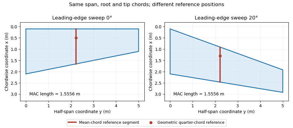
Identical trapezoidal chord distributions with different leading-edge sweep: the mean chord length stays fixed while its geometric reference position moves. Original calculation.
Details. Pinned article: Introduction to the OurBigBook Project
Welcome to the OurBigBook Project! Our goal is to create the perfect publishing platform for STEM subjects, and get university-level students to write the best free STEM tutorials ever.
Everyone is welcome to create an account and play with the site: ourbigbook.com/go/register. We belive that students themselves can write amazing tutorials, but teachers are welcome too. You can write about anything you want, it doesn't have to be STEM or even educational. Silly test content is very welcome and you won't be penalized in any way. Just keep it legal!
Intro to OurBigBook
. Source. We have two killer features:
- topics: topics group articles by different users with the same title, e.g. here is the topic for the "Fundamental Theorem of Calculus" ourbigbook.com/go/topic/fundamental-theorem-of-calculusArticles of different users are sorted by upvote within each article page. This feature is a bit like:
- a Wikipedia where each user can have their own version of each article
- a Q&A website like Stack Overflow, where multiple people can give their views on a given topic, and the best ones are sorted by upvote. Except you don't need to wait for someone to ask first, and any topic goes, no matter how narrow or broad
This feature makes it possible for readers to find better explanations of any topic created by other writers. And it allows writers to create an explanation in a place that readers might actually find it.
Figure 1. Screenshot of the "Derivative" topic page. View it live at: ourbigbook.com/go/topic/derivativeVideo 2. OurBigBook Web topics demo. Source. - local editing: you can store all your personal knowledge base content locally in a plaintext markup format that can be edited locally and published either:This way you can be sure that even if OurBigBook.com were to go down one day (which we have no plans to do as it is quite cheap to host!), your content will still be perfectly readable as a static site.
- to OurBigBook.com to get awesome multi-user features like topics and likes
- as HTML files to a static website, which you can host yourself for free on many external providers like GitHub Pages, and remain in full control

Figure 2. You can publish local OurBigBook lightweight markup files to either OurBigBook.com or as a static website.
Figure 3. Visual Studio Code extension installation.
Figure 5. . You can also edit articles on the Web editor without installing anything locally. Video 3. Edit locally and publish demo. Source. This shows editing OurBigBook Markup and publishing it using the Visual Studio Code extension. 
- Infinitely deep tables of contents:



All our software is open source and hosted at: github.com/ourbigbook/ourbigbook
Further documentation can be found at: docs.ourbigbook.com
Feel free to reach our to us for any help or suggestions: docs.ourbigbook.com/#contact