Topics (384k) Articles (398k) Users (410) Discussions (242) Comments (383) Files (13k) New article

Intensity interferometry infers source coherence from correlations between measured intensities, rather than directly combining electric-field amplitudes. For stationary chaotic Gaussian light, the normalized correlations satisfy , under the relevant statistical assumptions.
Separated detectors can therefore measure the magnitude of spatial coherence, which is related to the source's angular structure. Optical carrier phase need not be stabilized as in amplitude interferometry, but fast timing and sufficient photon statistics are crucial. The squared magnitude does not by itself retain every phase needed for unrestricted image reconstruction.
Phase-shifting interferometry measures an optical phase difference by recording light intensities at controlled relative wave phase shifts. For two sufficiently coherent fields at one detector point, a common model iswhere is a common background, a modulation amplitude and a known applied step. Several measurements separate the unknown wave phase from light intensity background and contrast; a single bright or dark frame generally cannot do so.
A concrete primary implementation was reported in 1974. A piezoelectrically varied reference arm and a 1024-element photodiode array supplied sampled light intensities to a minicomputer, which recovered wave phase by synchronous Fourier-series detection. The paper describes optical-surface and lens testing, repeated sampling and compensation of instrumental wavefront errors.[ref]
Digital Wavefront Measuring Interferometer for Testing Optical Surfaces and Lenses by J. H. Bruning and others. Abstract and p. 2693, apparatus and phase-detection method
This is an experimental implementation of controlled wave phase modulation; it is not a claim that every such system uses the same number of steps.Writing the model asturns wave phase recovery into a linear fit followed by . The step choices must make the three columns independent. Repeating only the same wave phase cannot identify all three unknowns. With more steps, least squares can fit the coefficients while exposing model residuals.
A reflecting reference mirror moved axially by changes its round-trip optical path by in the simple normal-incidence geometry, giving . A quarter-cycle wave phase step thus corresponds to ; at 632.8 nm this is 79.1 nm. These are geometric model values, not a calibration result for the historical apparatus.
Phase-step calibration error, light intensity drift, motion between frames and detector nonlinearity can all break the common-intensity model. The retrieved wave phase remains modulo , so phase unwrapping requires additional spatial or temporal information. The useful observable is the relative wave phase under controlled acquisition conditions, not an absolute optical wave phase inferred from brightness alone.
Phase unwrapping reconstructs a wave phase field from measurements that determine only its value modulo . If a detector or complex-argument calculation returns , then all values with integers give the same wrapped observation. Recovering a continuous wave phase therefore requires information beyond each isolated value. A primary 1982 analysis discusses this problem in wave phase curves obtained from image Fourier transforms before averaging them.[ref]
Analysis of the phase unwrapping algorithm by Kazuyoshi Itoh. Primary abstract, phase ambiguities and tracking motivation
Define with principal interval . If adjacent true differences satisfy , thenStarting from one reference wave phase, adding these wrapped differences reconstructs the sampled wave phase up to a global multiple of . The proof is direct: wrapping the two endpoint phases changes their difference only by an integer multiple of , and the strict bound selects its unique representative.
For an original example, true phases wrap to . Their wrapped increments are all , so reconstruction succeeds. But true increments produce exactly the same wrapped samples as increments . No algorithm can distinguish those two possibilities from the samples alone without a further assumption. Increasing sampling density can restore the bound only when the field's variation and noise allow it.
In two dimensions, different integration paths introduce a consistency test. A nonzero integer multiple of in the sum of wrapped increments around a closed sampling loop is a phase-unwrapping residue. Noise, undersampling or true wave phase singularities can obstruct a single consistent smooth reconstruction. Choosing an integration path is therefore part of the inference.
For interferometry, low interference visibility can make the wave phase poorly determined even before unwrapping. Unwrapping does not recover information lost where the measured complex amplitude vanishes, nor does it distinguish an actual discontinuity from a smooth but insufficiently sampled change. Report the wave phase reference, principal interval, sampling and any continuity assumptions alongside the reconstructed field.
A third-order intensity autocorrelation measures the delay-dependent intensity productThe name counts three intensity factors. A physical implementation can use two second-order nonlinear processes: second-harmonic generation creates a gate proportional to , and sum-frequency generation mixes it with a delayed fundamental replica. It therefore need not use a third-order material susceptibility. The historical device spatially encoded delay in crossing beams and imaged the sum-frequency signal onto a charge-coupled device.[ref]
A Single Shot 3rd Order Cross-Correlator for Pulse Contrast and Pulse Shape Measurements by J. Collier and others. printedpp194–195, equation forA3, Description and Figure2
An original Gaussian calculation illustrates response width. Set . Completing the square in the integral givesHence the third-order correlation width of a Gaussian pulse obeys for intensity full widths at half maximum. A correlation width would imply within this ideal Gaussian model. The square-root-of-two conversion appropriate to second-order Gaussian intensity autocorrelation would be different.
For a general pulse, need not equal ; this asymmetry can distinguish a delayed feature from an earlier one. It is still a cross-correlation with a finite-width nonlinear gate, rather than a direct reading of . The existing optical pulse temporal contrast derivation shows how a delayed weak replica also produces an opposite-delay third-order pulse correlation ghost.
Characterize phase matching, beam overlap, spatial uniformity and the temporal response before interpreting a narrow feature. Scaling the input intensity by scales this ideal signal by , so input fluctuations also matter. The measured trace does not uniquely reconstruct an arbitrary complex optical electric field.
The integrating-sphere escape probability is the chance that a photon in a specified integrating sphere model eventually leaves through a port rather than being absorbed by the wall. It depends on both the port area fraction and wall reflectance , as well as where the model begins. In the ideal uniformly diffuse model with nonreflecting ports, the integrating-sphere port-loss factor is and the survival probability between successive wall encounters is .[ref]
Integrating Sphere Theory and Applications by Labsphere. §1.2, printed p. 2, equations 6–12; §1.2.2, zero port reflectance versus general average reflectance
Start immediately before a wall encounter. The photon is absorbed there with probability , reflects and escapes before the next wall encounter with probability , or returns to the wall with probability . These satisfy . Under the same well-mixed encounter rule each time, eventual escape at encounter has probability . Summing the geometric series givesSimilarly, and . These are an original probability derivation of the guide's repeated-reflection bookkeeping, not an additional source of optical energy.
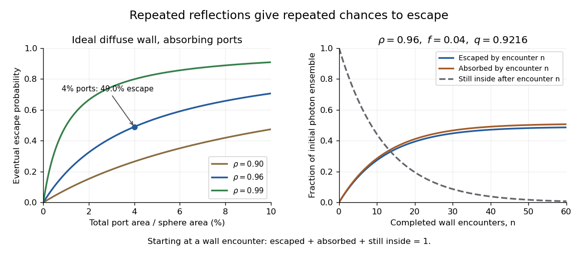
Ideal photon accounting from the first wall encounter: eventual escape versus port fraction, and cumulative escape, absorption and survival for a stated reflectance and port fraction
. Details. For an original numerical example, and give , soAlthough only four percent of the spherical area is open, almost half the initial photon ensemble eventually exits: surviving photons get repeated opportunities. After completed encounters, the escaped fraction is , the absorbed fraction is , and the fraction still inside is . The three fractions sum to one for every .
The stopping encounter has a geometric distribution with termination probability . Its expected count is , about 12.76 in this example. This counts wall encounters; it does not specify elapsed time without a model of path lengths and propagation.
Boundary cases clarify the assumptions. With and , every photon is eventually absorbed. With and , every photon eventually escapes. If both and , the ideal photon never terminates and the formula's is inapplicable. Starting after a successful first reflection instead would also give a different conditional escape probability; the starting point must accompany the result.
A measurement can vary a known aperture while injecting a stable radiant flux that first strikes the wall. A monitored detector then tests the apparatus response against a model including its viewing geometry. A single detector signal is not automatically the total energy escaping through all ports. Real coatings, reflective port fixtures and direct paths require corrections; baffles prevent the receiver from directly viewing an unusually bright first-illumination patch.[ref]
Integrating Sphere Theory and Applications by Labsphere. §1.2.2, average reflectance; §2.3, baffles and detector field of view
The probability above is therefore a useful ideal-model prediction, not a universal detector efficiency.An integrator reset establishes the charge on an integrating amplifier's feedback capacitor before the next measurement. Without it, the next output includes the previous initial condition, and repeated input pulses or input offset voltage can eventually cause amplifier clipping. Resetting makes consecutive measurement intervals comparable; it does not reconstruct a pulse already lost to amplifier clipping.
Consider an inverting integrating amplifier with the input held at zero during reset. Place an analog switch across its feedback capacitor . In the approximation of a stable ideal operational amplifier maintaining a virtual ground, a closed switch with constant on-state electrical resistance gives the RC circuit relationThis exponential decay gives an integrator reset settling time for residual magnitude at most :For stipulated values , and , the reset time constant is . Reaching a residual of requires about in this model. Actual amplifier drive, stability and recovery from overload can change the response. A switch's control delay also differs from the full circuit's settling time.[ref]
MT-088: Analog Switches and Multiplexers Basics. pp11–13, Figures19–21: settling versus switching delay
Opening the reset switch can itself disturb the initial condition. Analog switch charge injection transfers a small charge to the connected capacitor, producing a reset charge-injection pedestal of magnitudeFor a stipulated deposited on , this step is . Its sign depends on the circuit and charge direction. A longer reset suppresses the preceding exponential residual but need not suppress the new step created when the switch opens. Analog Devices illustrates this capacitive coupling mechanism and the resulting output step separately from retained-charge settling.[ref]
MT-088: Analog Switches and Multiplexers Basics. pp9–10, Figures13–16
A practical experiment repeats zero-input measurements with several reset durations and reads the output at the same delay after switch opening. A decreasing residual indicates incomplete discharge; a persistent offset can instead include reset charge-injection pedestal, input offset voltage and subsequent drift. Repeated readings help separate the reproducible offset from noise. The ACF2101 provides a concrete historical implementation: separate hold and reset controls disconnect the input and discharge the integration capacitor, and its datasheet shows the sequence of hold, integration and reset states.[ref]
ACF2101 Low Noise, Dual Switched Integrator datasheet. p9, Modes of Operation, Hold and Reset Switches, Figures3–4; p3, Charge Transfer Errors
The reset interval also creates integrator reset dead time: charge arriving while the circuit is being reset may not contribute to the next measured integral. Pulse timing relative to the reset therefore matters. A perfectly repeatable baseline alone does not establish that every input pulse was captured.
The amplifier input common-mode range is the set of common-mode voltages for which an electronic amplifier meets its operating requirements at the specified differential input, gain, supplies and load. A high common-mode rejection ratio describes rejection within a usable operating region; it does not extend that region. An instrumentation amplifier can have saturated internal stages even when its ideal final output fits the amplifier output range.[ref]
A Practical Review of Common Mode and Instrumentation Amplifiers by Eamon Nash. Three Op-Amp Instrumentation Amplifier, Common Mode Range, Figure5
An original simplified three-amplifier model makes the constraint visible. Let the input-stage output potentials bewhere and . Suppose each internal output must stay between and . ThenFor and , the permitted common interval is –. Choosing predicts internal outputs and and violates the stipulated limit. A unity-gain difference stage with reference would nevertheless predict a plausible final . That final prediction alone is insufficient.
This is an illustrative architecture model, not a device specification; input-device limits can impose further restrictions. A practical test holds fixed while sweeping both inputs together, recording differential gain error and distortion. Repeat at the intended gain and differential amplitudes. The resulting operating region is more informative than a single common-mode interval quoted without its test conditions.
An induced signal gain is the smallest norm-based amplification bound obtained by taking the worst case over admissible inputs. For a zero-initial-state operator satisfying ,For a linear map this is an operator norm between the specified normed spaces. Axler's definition takes the supremum of output norm over inputs of norm at most1, which is equivalent by linear scaling.[ref]
Linear Algebra Done Right by Sheldon Axler (4th edition). §7F, norm characterization7.88, printedp282
The norms are part of the definition. An original finite-dimensional example usesWith the same maximum-component norm at input and output, , and attains the ratio2. With the Euclidean norm, the Cauchy-Schwarz inequality gives , with equality at . With the sum-of-absolute-components norm, , and attains ratio1. The same matrix therefore has induced gains2, and1 under these three conventions.
For a time-dependent signal, the choice may additionally compare peak amplitudes or integrated squared amplitudes. The example in input-output gain derives a sharp peak-amplitude bound for a scalar dynamic system. A large response to one trial input supplies a lower bound on induced gain; proving a universal upper bound requires controlling every admissible input.
Compatible induced bounds compose. If and , thenThe intermediate norms must be the same. This inequality bounds a cascade without requiring the inputs that maximize the individual blocks to be simultaneously realizable, so the product need not be sharp. In robust performance, both the signal norms and the allowed control model uncertainty must be stated before such a bound can be interpreted.
Input capacitance describes the capacitive part of an electrical port's small-signal input impedance, under stated bias, frequency, and termination conditions. In a simple parallel model with the convention, its electrical admittance isThe electric current drawn by the capacitance grows with angular frequency even if the DC input resistance is enormous. Analog Devices distinguishes differential input paths from common-mode paths to ground: a quoted capacitance must identify which terminals are driven and how the remaining circuit is connected.[ref]
MT-040: Op Amp Input Impedance by Analog Devices. Printed p. 1, Figure 1, differential and common-mode input paths; printed p. 2, Op Amp Input Capacitance
For an original loading example, let and . At , the capacitive reactance magnitude is only . A source with electrical resistance therefore has loaded-to-unloaded phasor ratioThe DC ratio is about . Thus a resistance-only reading would miss a substantial high-frequency amplitude reduction. The numbers are chosen examples, not a specification for a named device.
For this same model, the source-to-input time constant is and the DC-normalized half-power signal bandwidth is its reciprocal divided by . A complex-error requirement is instead governed by capacitive bridging complex-error bandwidth; these specifications answer different questions.
For input capacitance inferred from measured admittance, apply a small sinusoidal electric potential difference, measure the input electric current and its phase shift, and infer within the parallel-capacitance approximation. Fixture, cable, and probe capacitances contribute to the measured port unless removed or included explicitly. Dependence on bias or frequency can make a single fitted an inadequate model.
Indole-3-acetate is the conjugate base of indole-3-acetic acid, formed by loss of a proton from its carboxylic acid group. ChEBI records molecular formula and charge . The uncharged acid and its anion have related chemical roles but are distinct protonation forms.[ref]
Write the acid as and indole-3-acetate as :For a dilute two-form model, the Henderson-Hasselbalch equation gives , and the anion fraction is . At pH equal to , the two fractions are equal. One pH unit above it gives anion, while one unit below gives . This is a symbolic calculation relative to the acid dissociation constant, not a claim of a newly measured numerical .
Oxygen consumption calorimetry estimates combustion heat release rate from the rate at which a fire consumes oxygen. Its practical usefulness comes from an approximate regularity: many common combustible materials release roughly per kilogram of consumed oxygen. The coefficient is an empirical energy equivalent for an applicable class of fuels, not a universal physical constant.[ref]
Standard Practice for Full-Scale Oxygen Consumption Calorimetry Fire Tests (ASTM E2067-20) by ASTM International. Public Significance and Use, §4.1: approximate energy release per unit mass of consumed oxygen
Let be the consumed oxygen mass flow rate, obtained from a consistent incoming/outgoing gas balance. A simplified model isFor an illustrative measured consumption rate of , this model givesThe observable must include gas throughput: an oxygen fraction by itself cannot determine a consumed mass per unit time.
In an exhaust-collection apparatus, a hood captures combustion products together with entrained air. Measurements of exhaust flow and gas composition allow the consumed oxygen rate to be inferred despite dilution. Gas sampling, mixing and the flow measurement must represent the same stream; gas amounts also need consistent wet/dry conventions and reference temperature and pressure. The NIST National Fire Research Laboratory uses exhaust systems to measure large-fire heat release rate by this principle.[ref]
National Fire Research Laboratory by NIST. Facility description, exhaust collection and oxygen-consumption calorimetry
[ref]Standard Practice for Full-Scale Oxygen Consumption Calorimetry Fire Tests (ASTM E2067-20) by ASTM International. Public Significance and Use, §4.3: oxygen concentration and exhaust-flow measurements
A useful experimental check is an independently metered reference burner. Its fuel-consumption-based energy input can be compared with the heat release rate inferred from oxygen depletion; NIST describes natural-gas burners for this mutual confirmation. This tests the measurement chain rather than merely exposing a gas analyzer to a known mixture.[ref]
Natural Gas Confirmation Burner by NIST. Research Overview, comparison of fuel-consumption and oxygen-consumption calorimetry
Incomplete capture, changing fuel composition, incomplete combustion and analyzer transport delays can all affect the inferred curve. They concern different parts of the inference: lost exhaust biases the gas balance, an inappropriate energy equivalent changes the conversion, and delayed sampling shifts the response in time. A reported heat release rate therefore needs both its conversion assumptions and its measurement conditions.
An inclusion indicator records whether a specified population unit appears in a sample :It is an indicator random variable, with expected value and variance . Its randomness comes from sample selection; the population value attached to unit may be treated as fixed in a sampling calculation.[ref]
Unequal Probability Sampling in Penn State STAT 506. Lesson 3, inclusion probabilities and inverse-probability total estimation
Inclusion indicators turn a sum over a changing sample into a sum over fixed population labels:If every , the same identity immediately provesThe inverse-inclusion-probability total is unbiased because , not because the selected units must look typical in every realization.
Pair products connect the notation to joint inclusion probabilities: , so . For a fixed sample size , in every realization. Consequently,In simple random sampling with , the four individual variances sum to , while the six distinct pair covariances are each . Their doubled sum is , giving total variance zero. Treating the inclusion indicators as independent would incorrectly predict a random sample size. The notation makes that error easy to detect.
A joint inclusion probability is the probability that two specified population units both belong to a random sample :For the same unit twice, , where is its inclusion probability. For distinct units, is generally not : selection can make their inclusion indicators dependent. These probabilities describe the sampling procedure, rather than a relationship between the measured values of the two units.[ref]
Unequal Probability Sampling in Penn State STAT 506. Lesson 3, inclusion probabilities and finite-population estimation
For simple random sampling of distinct labels from labels, counting subsets containing both and giveswith value zero if . Since ,For , each unit has inclusion probability , but a particular pair has joint inclusion probability . Conditional on including one member, the other is included with probability , not .
Equal individual inclusion probabilities do not determine these pair probabilities. A different procedure that chooses only or , each with probability , still includes each unit with probability . Yet and . Thus two procedures can agree on individual representation while producing different dependence and different precision for a population summary. The distinction motivates keeping pair information when calculating the variance of weighted survey estimators; the classical general treatment is due to D. G. Horvitz and D. J. Thompson.[ref]
A Generalization of Sampling Without Replacement From a Finite Universe by D. G. Horvitz and D. J. Thompson. Publisher abstract and original publication, pp. 663–685
An impedance-head mass correction removes the inertial force required to accelerate material between an impedance head's force-sensing plane and the specimen. The manufacturer's construction places the acceleration sensor above the force gauge and makes the connection to the driving point stiff. Its guidance recommends compensation when the specimen's mechanical dynamic mass is comparable to the mass below the gauge.[ref]
Choose a common positive axis and assume a rigid intervening mass shares specimen acceleration . Newton's second law givesHere are synchronized complex amplitudes at the same angular frequency. Hence the corrected mechanical dynamic mass is , and corrected mechanical accelerance is . The effective intervening mass must include the applicable mounting hardware; it is not automatically the entire sensor mass.
For an original example, take , real, and . Then , with magnitude . Subtracting unsigned amplitudes would instead give and lose the correct phase. The corrected mechanical dynamic mass is .
The model requires synchronized channels, appropriate measurement calibration and sufficiently rigid motion below the force gauge. If that assembly flexes, its motion cannot be represented by one frequency-independent . Subtracting inertia also does not recover the unattached specimen's response: the attached head can still change its natural frequencies and mode shapes. A useful apparatus check is a rigid test mass, for which the force/acceleration ratio should agree with the total moving mass in the chosen force plane within the tested range.
Impedance bridging with capacitive input treats a receiver's input as a resistance in parallel with a capacitance. Even when its DC input impedance is large, the capacitive path can draw appreciable electric current at higher frequency, changing both the amplitude and phase of the observed electric potential difference.
For source resistance , receiving resistance and input capacitance , use sinusoidal steady-state phasors and a linear source model. The receiving electrical admittance is , soHere is the open-circuit source phasor; is the loaded terminal phasor. The impedance bridging objective is near one, rather than merely a large quoted DC input resistance.
The amplitude and phase responses areAn amplitude-only tolerance and a tolerance on the full complex number express different requirements. The latter measuresFor positive resistances, capacitance and a chosen , the capacitive bridging complex-error bandwidth condition requiresA negative numerator means even the DC loading error exceeds the tolerance.
In an original example, , and give . A one-percent complex-error tolerance permits frequencies only up to about . At the amplitude ratio remains about , but the phase is about and the complex error about . A small amplitude error can coexist with a materially larger waveform-phase error.
High-input-impedance buffers are motivated by just this source-loading problem. Texas Instruments' three-amplifier presentation shows how current drawn from a source with finite output impedance degrades accuracy and how input buffers reduce loading.[ref] The chosen component values above are not specifications of a particular amplifier. A real receiver may require additional input paths, frequency-dependent source impedance and a model of the connected cable or probe.
A dye-loss interaction is a departure from additivity on a specified response scale. Changing from fractional loss to survival, logarithmic survival or a fitted rate can change that departure. The contrast must therefore be defined before it is interpreted as evidence about coupled chemical mechanisms.
For a crossed initiation/illumination experiment, write fractional losses at a common observation time and defineAn original example takes losses . The contrast is . Yet the surviving fractions obey , with . They are exactly multiplicative on the survival scale.
For first-order survival , transform to . The rate-scale interaction isThe example gives . More generally, additive rates yieldwhich is negative for positive . The fractional-loss ceiling creates the contrast without an additional rate interaction.
The transformation also changes noise. First-order uncertainty propagation gives , so near-complete loss can strongly amplify uncertainty. In addition, the mean of a nonlinear transformation need not equal the transformation of the mean; Jensen's inequality makes that distinction explicit. Averaging transformed replicates and transforming an average need not produce the same result.
The STY-BODIPY readout is a coupled oxidation signal. Its primary method distinguishes radical-trapping kinetics from stoichiometry.[ref]
A Continuous Visible Light Spectrophotometric Approach To Accurately Determine the Reactivity of Radical-Trapping Antioxidants by Evan A. Haidasz and others. Abstract, co-autoxidation method and kinetic/stoichiometric interpretation
A rate transformation requires a justified survival model after product absorption and background have been addressed. Report both the response definition and the uncertainty model; a transformed zero is conditional evidence about that model, rather than a unique identification of the chemistry.An idler support reaction is the force exerted by the shaft and bearings that balances the mesh loads and other external loads on an idler gear. A vanishing net transmitted torque does not imply a vanishing resultant force: moments can cancel while forces add. A free-body diagram must retain each tooth-contact force and its point of application. The tangential load in each ideal mesh follows from .[ref]
Elements of Metric Gear Technology by SDP-SI. §7, gear forces; tangential transmitted load and pressure-angle separation of mesh forces
Consider a steady collinear train with input, idler and output reference radii20,30 and50mm. An input torque gives a100N tangential mesh component. On the idler, choose contact positions at and relative to its center, with both tangential forces upward. Their moments are and , but their vector sum is200N upward. For equal20degree pressure angles, the two radial mesh components have magnitude and opposite directions, so they cancel. Neglecting other loads, the net support reaction is200N downward.
This is the combined support resultant, not automatically the load on each bearing. For a hypothetical shaft supported at axial positions and , with the200N upward gear resultant acting at , static equilibrium givesThus and . Idler bearing load sharing depends on placement even when the total reaction is fixed.
Noncollinear shaft layouts rotate the mesh-force directions, and helical gears add gear axial force. Acceleration also changes the balance: the sum of torques must supply the idler's angular acceleration, and unequal mesh loads need not cancel radially. The zero-net-torque example therefore establishes a steady ideal force balance, rather than a universal bearing-load formula.
A hypophyseal portal vein is a vein connecting the first and second capillary networks of the hypophyseal portal system. The main route carries blood from the median eminence region of the hypothalamus, down the pituitary stalk, to the anterior pituitary. It delivers hypothalamic hormones before their dilution in the wider circulation.[ref]
Anatomy and Physiology 2e by J. Gordon Betts and others. Section17.3, Anterior Pituitary and Figure17.9: primary plexus, portal veins and secondary plexus
The word “portal” describes the route: blood leaving one capillary bed reaches another capillary bed before returning to the heart. Here the first bed receives a regulatory message and the second delivers it to responding biological cells. A hypophyseal portal vein is therefore an interconnecting segment, rather than the entire hypophyseal portal system.
A useful example is a pulse of gonadotropin-releasing hormone. In conscious sheep, simultaneous sampling of portal and peripheral blood plasma linked portal GnRH pulses with peripheral luteinizing hormone episodes. Sampling the hypophyseal portal vein route accesses the incoming hypothalamic signal; peripheral sampling detects the resulting pituitary output. That distinction is why the sampling location is part of the experiment, not just a convenient place to draw blood.[ref]
The temporal relationship between gonadotropin releasing hormone (GnRH) and luteinizing hormone (LH) secretion in ovariectomized ewes by Iain J. Clarke and James T. Cummins. Abstract: synchronized portal GnRH and peripheral LH secretion in conscious ovariectomized ewes
Pinned article: Introduction to the OurBigBook Project
Welcome to the OurBigBook Project! Our goal is to create the perfect publishing platform for STEM subjects, and get university-level students to write the best free STEM tutorials ever.
Everyone is welcome to create an account and play with the site: ourbigbook.com/go/register. We belive that students themselves can write amazing tutorials, but teachers are welcome too. You can write about anything you want, it doesn't have to be STEM or even educational. Silly test content is very welcome and you won't be penalized in any way. Just keep it legal!
Intro to OurBigBook
. Source. We have two killer features:
- topics: topics group articles by different users with the same title, e.g. here is the topic for the "Fundamental Theorem of Calculus" ourbigbook.com/go/topic/fundamental-theorem-of-calculusArticles of different users are sorted by upvote within each article page. This feature is a bit like:
- a Wikipedia where each user can have their own version of each article
- a Q&A website like Stack Overflow, where multiple people can give their views on a given topic, and the best ones are sorted by upvote. Except you don't need to wait for someone to ask first, and any topic goes, no matter how narrow or broad
This feature makes it possible for readers to find better explanations of any topic created by other writers. And it allows writers to create an explanation in a place that readers might actually find it.
Figure 1. Screenshot of the "Derivative" topic page. View it live at: ourbigbook.com/go/topic/derivativeVideo 2. OurBigBook Web topics demo. Source. - local editing: you can store all your personal knowledge base content locally in a plaintext markup format that can be edited locally and published either:This way you can be sure that even if OurBigBook.com were to go down one day (which we have no plans to do as it is quite cheap to host!), your content will still be perfectly readable as a static site.
- to OurBigBook.com to get awesome multi-user features like topics and likes
- as HTML files to a static website, which you can host yourself for free on many external providers like GitHub Pages, and remain in full control

Figure 2. You can publish local OurBigBook lightweight markup files to either OurBigBook.com or as a static website.
Figure 3. Visual Studio Code extension installation.
Figure 5. . You can also edit articles on the Web editor without installing anything locally. Video 3. Edit locally and publish demo. Source. This shows editing OurBigBook Markup and publishing it using the Visual Studio Code extension. 
- Infinitely deep tables of contents:



All our software is open source and hosted at: github.com/ourbigbook/ourbigbook
Further documentation can be found at: docs.ourbigbook.com
Feel free to reach our to us for any help or suggestions: docs.ourbigbook.com/#contact