A proteoliposome is a liposome containing one or more reconstituted membrane proteins in its lipid bilayer. It combines a controlled membrane boundary with a chosen molecular machine. A solution containing detergent-solubilized protein is not automatically a proteoliposome: a closed vesicle and a membrane-incorporated protein must actually be formed.

The artificial compartment is useful because material can be placed on one side of a lipid bilayer and transport measured across it. In an originating experiment on the NhaA sodium/proton antiporter, purified protein was reconstituted into sodium-loaded proteoliposomes. Parallel sodium and proton flux measurements, together with an independent membrane-potential equilibrium method, supported a stoichiometry of two protons per sodium ion over the tested pH range 7.2–8.1.^[ref]

For a bookkeeping example,100 sodium ions moved outward through a perfectly coupled $2{\mathrm{H}}^{+}/\mathrm{N}{\mathrm{a}}^{+}$ exchanger would accompany 200 protons moving inward. The net movement is 100 positive elementary charges inward, which explains the word electrogenic. These invented counts illustrate coupling, not a measured single-vesicle trace.

Interpreting a proteoliposome assay still requires knowing which way the membrane protein faces, whether the vesicles leak, and how much protein is incorporated. An otherwise matched empty liposome helps estimate membrane background. Reconstitution simplifies a biological system; it does not automatically eliminate every alternative source of the measured flux.

Dynamic character-device number allocation asks the Linux kernel to reserve a range of character-device numbers while choosing its major device number at runtime. The API is alloc_chrdev_region(dev_t *dev, unsigned baseminor, unsigned count, const char *name). It returns zero on success or a negative error code; the first assigned combined device number is written through dev. The return status is not the allocated major number.^[ref]

For an original request, suppose alloc_chrdev_region(&first, 5, 3, "sample") succeeds and the returned first has major $M$. Its reserved identifiers are $(M,5)$, $(M,6)$ and $(M,7)$, not $(M,8)$. If one illustrative successful run returned major 243, the caller would use 243; another allocation can return a different major. This is a hypothetical range example, not a kernel operation executed here.

Keep first and the successful reservation count for cleanup. If a later initialization step fails, unregister_chrdev_region(first, 3) releases this reservation; it must not be treated as ownership of every minor under the returned major. Unwinding a failed character-device registration releases only resources actually acquired.

Number reservation is separate from associating file operations with a live character-device object and from creating a device node. The related cdev_add operation makes a registered object live; its name or bookkeeping label does not itself establish a pathname under /dev.^[ref]

Removal must also respect existing users. cdev_del prevents new opens, but already open file descriptors can still call device operations, so deleting the registration alone does not prove that backing state can be freed immediately.^[ref] A dynamic number is a reserved interface identifier, not a persistent hardware identity or an inode number.

A direct linear solver computes the solution of a finite linear system by a fixed sequence of algebraic eliminations or matrix factorizations, rather than successive approximate iterates until a stopping tolerance is met. For a nonsingular square matrix, a typical method uses Pivoted LU decomposition followed by forward and back substitution.

For $2x+y=1$ and $x+3y=2$, subtracting half the first row from the second gives $(5/2)y=3/2$. Hence $y=3/5$ and $x=1/5$. Elimination produces a triangular system whose unknowns are recovered in reverse order.

The adjective direct describes the method's finite algebraic structure; floating-point computation still incurs roundoff. Pivoting avoids unusable or dangerously small pivots, while the condition number controls how perturbations can affect the answer. Factoring a matrix once and reusing the factors can efficiently handle many different right-hand sides.

The general Heun equation is the second-order linear ordinary differential equationIt is a canonical Fuchsian equation with four singular locations $0,1,a,\infty$, generically all regular singular points. Special parameter choices can make some singularities apparent or removable. The local exponent pairs are $(0,1-\gamma )$, $(0,1-\delta )$, $(0,1-ϵ)$ and $(\alpha ,\beta )$, respectively.^[ref]

The parameter $a$ locates the fourth singularity, while $q$ is an accessory parameter not fixed by those local exponent pairs. For instance, setting $\alpha =q=0$ makes the constant function $w=1$ a solution, as direct substitution shows. Coalescing singularities gives confluent Heun equations with different singularity structures; these are not the same four-distinct-point equation. Heun functions supply named solutions for boundary-value problems beyond the three-singularity hypergeometric case.

An unbounded operator is a linear map $T:D(T)\subseteq X\to Y$ for which no finite constant $C$ bounds $\Vert Tx{\Vert }_Y\le C\Vert x{\Vert }_X$ on its domain. The domain and norms are therefore part of its specification.

On complex $L^2(0,2\pi )$, take $T=-id/dx$ with periodic $H^1$ domain. The functions $e_n(x)=e^{inx}/\sqrt{2\pi }$ have norm one, while $T{e}_n=n{e}_n$ has norm $|n|$. Hence no such constant exists. Differentiation can nevertheless be bounded when the source is equipped with an $H^1$ norm. An operator's unboundedness thus cannot be inferred from its formula without stating the spaces and domain.

For a function $f:D\to Y$ between metric spaces, and an accumulation point $a$ of $D\subseteq X$, the limit of a function satisfies ${\lim }_{x\to a}f(x)=L$ exactly when every sequence $x_n\in D\setminus \{a\}$ converging to $a$ has $f(x_n)\to L$.

The forward implication substitutes eventual closeness of $x_n$ into the epsilon-delta condition. For the converse, if that condition fails, some ${\epsilon }_0>0$ permits a choice of $x_n$ withThis sequence approaches $a$ while its images fail to approach $L$, a contradiction.

For $f(x)=\sin (1/x)$ near zero, take $x_n=(2\pi n+\pi /2{)}^{-1}$ and $y_n=(2\pi n+3\pi /2{)}^{-1}$. Both sequences tend to zero, but their images are $1$ and $-1$. Hence the limit of a function does not exist there. The metric-space hypothesis matters: sequences do not detect all limits in arbitrary topological spaces.

An organic light-emitting diode produces light when injected electrons and electron holes recombine in an organic emitting layer. Contacts and transport layers bring the two charge-carrier types together; radiative relaxation of the resulting excited states supplies the emitted photons. The device is emissive, so an individual display pixel can generate its own light.

The 1987 two-layer device used an indium tin oxide anode, an organic hole-transport layer, an aluminum-chelate emitting layer and a magnesium-silver cathode. Electrode choice and the organic interface confined recombination to the emitting region. Measuring current and escaping light separately distinguished charge injection from useful optical output.^[ref]

The span efficiency factor $e$ compares a wing’s lift-induced drag with a reference induced-drag level at the same lift, span and dynamic pressure. In the conventional finite-wing coefficient model,It describes the induced contribution under stated geometry and flow assumptions. NASA’s primary account gives this relation and identifies the elliptic-load ideal in its lifting-line discussion.^[ref]

For an ideal planar wing in classical lifting-line theory, elliptic span loading minimizes induced drag for fixed lift and span, corresponding to $e=1$ in this normalization. Deviations of the loading can increase induced drag and lower $e$. The load distribution depends on twist, section properties and operating conditions as well as planform. An outline alone therefore does not specify a universal efficiency value. Nonplanar systems and different reference conventions require their own interpretation before applying the planar bound.

For an original coefficient example, choose $C_L=0.80$, $AR=8$ and $e=0.80$. Then $C_{D_i}\approx 0.031831$. With $q_{\infty }=500\mathrm{Pa}$ and $S=20{\mathrm{m}}^2$, lift is $8000\mathrm{N}$ and induced drag is about $318.3\mathrm{N}$. At $e=1$ with those other quantities fixed, induced drag would be about $254.6\mathrm{N}$. Thus the chosen $e=0.8$ corresponds to a 25-percent induced-drag increase over that reference, not a statement that twenty percent of all input power is lost.

A drag-polar fit illustrates why efficiency definitions can differ. Suppose a model haswhere $k_v$ is an additional lift-dependent profile-drag coefficient and $e_i$ is the induced efficiency. Fitting the entire quadratic term as $C_L^2/(\pi AR{e}_{\mathrm{fit}})$ givesFor stipulated $e_i=0.90$, $AR=8$ and $k_v=0.010$, the fitted value is about $0.734$. The algebra does not identify $e_{\mathrm{fit}}$ with the induced-only factor. It shows how a total-drag fit can absorb another modeled contribution even when the induced flow itself has not changed.

The inversion is also sensitive to a small extracted drag. At fixed $C_L$ and $AR$, a small fractional error in $C_{D_i}$ gives approximately the opposite fractional error in $e$. If induced drag is obtained by subtracting a large estimated profile contribution from total drag, uncertainty in that subtraction can dominate. Different reference areas or lift conditions also change the comparison.

A proposed test combines measured lift and drag with a separately justified profile-drag estimate or a calibrated wake-based induced-drag inference. Repeat over the intended coefficient range and report the geometry, area convention, flow regime and uncertainty. A single fitted number is useful only alongside the model that separates induced drag from the rest of the measured aerodynamic force.

A wingtip vortex is a concentrated rotating part of the wake behind a finite lifting wing. Spanwise variation of the wing’s circulation produces trailing vorticity, which can roll up into a strong counter-rotating pair. The two rotating wakes induce downward motion between them and upward motion farther outside. NASA’s account connects the tip-region pressure-driven flow with the pair and its induced change of local flow direction.^[ref]

A useful idealization treats each concentrated wake as a straight line vortex. Outside its core, circular symmetry and the definition of circulation giveFor stipulated $|\Gamma |=20{\mathrm{m}}^2/s$ and $r=0.50\mathrm{m}$, the ideal tangential speed is about $6.37m/s$. The singularity as $r\to 0$ is a defect of the line model: a real vortex has a finite core and a nonuniform vorticity distribution.

Consider an original cross-flow model with cores separated horizontally by $d$, strengths $-\Gamma$ and $+\Gamma$, and orientations chosen to give downwash between them. Each ideal vortex induces downward speed $|\Gamma |/(2\pi d)$ at the other core. At $d=10\mathrm{m}$ and $|\Gamma |=20{\mathrm{m}}^2/s$, this pair-interaction speed is about $0.318m/s$. At the midpoint, adding their two velocities gives $2|\Gamma |/(\pi d)\approx 1.273m/s$ downward. These are distinct locations and distinct speeds.

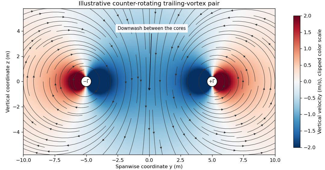
The wake is not generally two permanently straight tubes with fixed strength. A distributed trailing sheet rolls up, the cores move under induced velocities, and viscosity, turbulence and ambient motion alter the field. A wing’s actual span loading and operating state determine the wake, so the illustrative circulation and core size cannot be assigned to an aircraft merely from its visible span.

The connection to lift-induced drag is the complete induced-flow and load system. A short line sketched at each wingtip is not an extra independent friction force to add to an already complete drag calculation. The flow carries momentum and kinetic energy while changing the force direction experienced by the finite wing.

A proposed laboratory wake survey places a finite wing at a controlled load in a wind tunnel and measures transverse velocity at a downstream plane using calibrated directional probes or timed tracer images. Reverse the sign of lift to check the expected reversal of rotation, and compare measured circulation on several enclosing paths outside the cores. Tracers must follow the flow adequately, while finite sampling, tunnel walls and the probe’s own disturbance limit the inference. A visible tracer pattern alone does not supply the full three-dimensional velocity or pressure field.

Downwash is a downward component of fluid velocity, commonly the induced flow associated with a lifting wing and its trailing vortices. For positive upward lift, this flow changes the direction of the local relative wind and contributes to lift-induced drag. NASA's primary explanation connects the trailing vortex system, reduced effective incidence and rearward component of the aerodynamic force.^[ref]

Choose streamwise velocity $U>0$ and let $w>0$ denote downward induced speed at a section. The induced angle and effective angle of attack areAn ideal local lifting force normal to that relative flow is tilted rearward. Its vertical and downstream projections obey $D_i/L=\tan {\alpha }_i=w/U$; hence $D_i\approx L{\alpha }_i$ for small induced angles. This projection isolates the induced contribution in the stated model; it does not include skin friction or every source of total drag.

For an original uniform-downwash example, take $U=50m/s$, $w=2m/s$ and total lift $L=10000\mathrm{N}$. Then ${\alpha }_i\approx 2.291^{\circ }$ and $D_i=400\mathrm{N}$ in the projection model. The power required to overcome this contribution is $U{D}_i=20\mathrm{kW}$. At geometric incidence $6^{\circ }$, the effective incidence is about $3.709^{\circ }$.

A real finite wing generally has span-dependent loading and induced speed. In small-angle lifting-line theory,Using an unweighted arithmetic mean of measured $w$ need not reproduce that integral. For elliptic span loading, the ideal lifting-line downwash is constant across the span and ${\alpha }_i\simeq C_L/(\pi AR)$, consistent with $C_{D_i}=C_L^2/(\pi AR)$. These statements concern the ideal planar model rather than arbitrary wakes or separated flow.

A proposed observation measures flow direction and speed at a specified plane around a loaded wing, using calibrated directional probes or timed tracer images. Repeat with zero and reversed lift, and compare the sign and spatial distribution of the induced flow. Record the freestream reference and wing incidence as well as the probe positions. Wake-plane dependence of a downwash measurement matters: a velocity measured well downstream cannot simply be inserted as the wing-section induced speed without a model connecting the two planes. Visible tracer deflection demonstrates flow direction only to the extent that the tracer follows the fluid; it is not by itself a quantitative lift or drag measurement.

In the setting of a uniform pro-p group $G$, its integral Lazard Lie algebra is a finite free ${\mathbb{Z}}_p$-module whose addition and Lie bracket recover infinitesimal versions of group multiplication and the group commutator. It carries more integral information than the associated ${\mathbb{Q}}_p$-Lie algebra. The construction requires hypotheses on the group and its filtration; it is not available unchanged for every profinite group.^[ref]

For odd $p$, a concrete example is $G=1+p{M}_n({\mathbb{Z}}_p)$. The convergent matrix logarithm and matrix exponential identify its Lie algebra with $p{M}_n({\mathbb{Z}}_p)$, using ordinary matrix addition and bracket $[A,B]=AB-BA$. Multiplication corresponds to the Baker--Campbell--Hausdorff formula, beginningFor $p=2$, the analogous safe neighborhood is $1+4M_n({\mathbb{Z}}_2)$ with Lie algebra $4M_n({\mathbb{Z}}_2)$. The smaller neighborhood $1+2{\mathbb{Z}}_2$ contains $-1$, so torsion already prevents it from being uniform.^[ref]

For the additive group ${\mathbb{Z}}_p$, the associated Lie algebra is rank one with zero bracket. Under suitable coefficient hypotheses, the Lazard isomorphism compares its Lie algebra cohomology with continuous group cohomology.

Medicago truncatula is a legume widely used as a model organism for plant biology, particularly the association between rhizobia and root nodules. In this symbiosis, bacterial nitrogen fixation supplies biologically usable nitrogen within specialized plant structures. The plant and its microbial partners contribute different parts of the process.^[ref]

The 2011 draft genome study combined a large-insert assembly with additional short-read sequence data. Comparing duplicated genomic regions and genes with enhanced activity in root nodules helped investigate how gene duplication contributed to the evolution of this symbiosis.^[ref] A useful comparison asks whether both copies of a duplicated gene retain nodule-associated activity or whether their expression patterns differ. Sequence similarity identifies candidate relatives; measuring activity supplies another kind of evidence about their roles.

The same plant also supports questions outside nodule formation. In a 2005 study, fluorescence microscopy of green fluorescent protein-labelled Methylorubrum extorquens derivatives located bacterial cells on leaves and in some internal spaces.^[ref] This visualizes colonization. A fluorescent bacterium on a leaf does not by itself establish nitrogen fixation, nodule formation or a benefit to the host.

The local fixed point index assigns an integer to an isolated fixed point $a$ of a continuous map $f:U\to {\mathbb{R}}^n$, where $U$ is a neighbourhood of $a$. Choose a small ball $B$ containing no other fixed point; thenThe mapping degree counts the zero of the displacement map with its local topological multiplicity. Changing the ball or deforming $f$ without allowing a fixed point onto its boundary leaves this index unchanged.

If $f$ is differentiable and $I-Df(a)$ is invertible, the first-order displacement gives $i(f,a)=\mathrm{sign}\det (I-Df(a))$. On the real line, $f(x)=x/2$ has index $+1$ at zero, while $f(x)=2x$ has index $-1$ there. A nonzero index forces the existence of a fixed point in the region. Under the hypotheses of the Lefschetz-Hopf fixed-point theorem, the sum of local indices is the global Lefschetz number.

CSS leading is the extra allowance around the font ascent and font descent when CSS constructs the vertical extent associated with a glyph. Let $A$ be the positive ascent, $D$ the positive descent magnitude and $H$ the selected line height, all at the same font size and in the same units. The extra leading and the resulting extents above and below the text baseline areThe half-leading is a layout allocation. It need not be a visible blank strip, and $L$ may be negative.^[ref]

This explains a subtle effect of mixing fonts. In a simple baseline-aligned line containing only ordinary text CSS inline boxes, include the block's CSS strut among the contributions indexed by $i$. The CSS line box must extend far enough in each direction, givingThe two maxima can come from different contributions. Suppose one has $(A,D,H)=(11,3,18)$ CSS pixels, giving $(A^{\prime },D^{\prime })=(13,5)$, while another has $(8,4,20)$, giving $(12,8)$. If the CSS strut adds no larger extent, the resulting CSS line box is $13+8=21$ CSS pixels high, exceeding both declared line heights. The assumption of a common text baseline matters: other vertical alignments and inline objects require the fuller layout rules.^[ref]

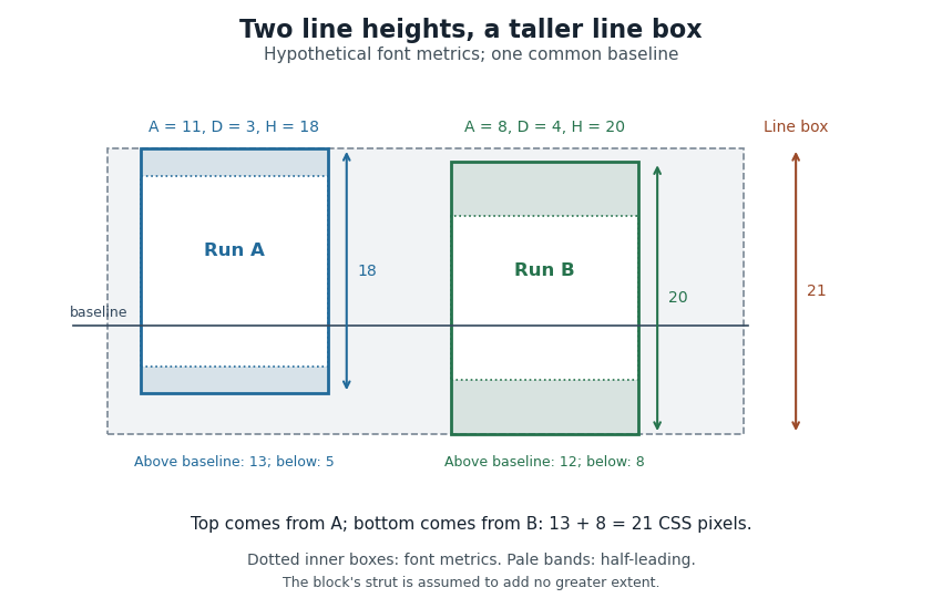
Thus a stored font line gap, an individual line height declaration and the final CSS line box height are distinct quantities. Comparing only nominal font sizes cannot explain the mixed-font result.

A primitive lattice vector is a nonzero element $u$ of a finite-rank free abelian group $N$ that cannot be written $u=kv$ with $v\in N$ and an integer $|k|>1$. In an integral basis, this is equivalent to the greatest common divisor of its coordinates being one. The property is independent of the chosen lattice basis.

For example, $(2,3)$ is primitive although neither coordinate is one: the integer functional $\ell (x,y)=-x+y$ satisfies $\ell (2,3)=1$. Hence $N=\mathbb{Z}u\oplus \ker \ell$, showing that $u$ extends to a lattice basis. In contrast, $(2,4)=2(1,2)$ is not primitive.

Every rational ray of a fan contains a unique primitive generator pointing along it. This generator gives the integral normalization used in toric divisors and cocharacters; replacing it by a larger positive multiple leaves the geometric ray unchanged but changes its lattice data.

A variational autoencoder is a generative model with a latent variable $z$ and a learned approximation to its posterior distribution given an observation $x$. Write the model as $p_{\theta }(x,z)=p(z)p_{\theta }(x\mid z)$. A recognition network, implemented as a neural network, produces the parameters of $q_{\varphi }(z\mid x)$; a generative decoder specifies $p_{\theta }(x\mid z)$. Using one recognition rule across observations is amortized inference, rather than solving a fresh independent optimization problem for every input.^[ref]

Training maximizes an evidence lower bound, often writtenThe first term scores reconstruction under the declared likelihood; the second compares the inferred latent law with the prior. The identityproves that it is a lower bound, since Kullback-Leibler divergence is nonnegative. It becomes tight when the recognition law equals the model posterior, under the usual density/support conditions.^[ref]

For a one-dimensional Gaussian example, let the prior be $N(0,1)$ and the recognition law be $N(\mu ,{\sigma }^2)$. Substituting their log densities and using $\mathbb{E}[z^2]={\mu }^2+{\sigma }^2$ givesAt $\mu =1$, $\sigma =2$, this is $2-\log 2\simeq 1.30685$. The value is a penalty for this particular latent law, not the whole training loss. Gaussian reparameterization writes $z=\mu +\sigma \epsilon$ with fixed-law standard-normal noise so that gradients can pass through the sampled latent value. After training, generation instead draws from the prior and then the generative decoder; it need not start from an observed input.

The Schilder theorem gives a large deviation principle for small Brownian motion paths. For standard Brownian motion $W$ starting at zero on $[0,T]$, the laws of $\sqrt{\epsilon }W$ on continuous paths with the uniform norm have speed $1/\epsilon$ and good rate functionIn particular, the zero starting value and finite-energy path class are part of the rate. Typical Brownian motion paths are not themselves absolutely continuous; the rate describes the exponential cost of neighborhoods of prescribed paths.^[ref]

For paths constrained by $\varphi (T)=b$, the Cauchy-Schwarz inequality gives ${\int }_0^T|\dot{\varphi }{|}^{2}dt\ge b^2/T$, with equality for $\varphi (t)=bt/T$. Thus the least endpoint cost is $b^2/(2T)$, agreeing with the exponential scale of the normal distribution of $\sqrt{\epsilon }{W}_T$.