The normal contact penalty time scale describes the fast dynamics introduced by a stiff normal-contact approximation. For a compressed linear penalty spring with stiffness $k$ acting on a point mass $m$, small oscillations about equilibrium satisfy $m\ddot{x}+kx=0$. Their angular frequency, reference time and period areThe reference time $t_c$ is not the full oscillation period. Rescaling time by $s=t/t_c$ gives $d^{2}x/d{s}^2+x=0$, so a numerical step is controlled by its dimensionless size $h/t_c$, not just its duration in seconds. The primary compliant-contact treatment highlights the numerical stiffness caused by such springs.^[ref]

A modeling and numerical budget interact. Limiting equilibrium overlap under a specified maximum supported load $F_{\max }$ to $d_{\max }$ requires $k\ge F_{\max }/d_{\max }$ in this linear model. For an original choice $F_{\max }=10\mathrm{N}$ and $d_{\max }=10\mu \mathrm{m}$, choose $k=10^6\mathrm{N}{\mathrm{m}}^{-1}$. At $m=0.5\mathrm{kg}$,A chosen resolution target of twenty steps per contact oscillation would set $h\le 0.2221\mathrm{ms}$. This is a resolution target, not a universal accuracy or stability theorem for every integrator.

Increasing the stiffness by a factor of 100 reduces the same-load overlap by 100 but reduces these times by only ten. Keeping the old step then gives roughly two samples per new oscillation instead of twenty. The parent penalty approximation of unilateral contact also shows why the Forward Euler method's undamped-oscillator instability cannot be cured merely by calling the step small.

For a multibody contact, the effective mass in a normal-contact penalty mode replaces an arbitrary total body mass. Additional damping and nonlinear force laws can introduce other time scales. A convergence study should therefore check force histories and contact events as well as maximum overlap; smaller geometric penetration alone does not establish a more accurate simulation.

Peak phasor versus positive-frequency Fourier coefficient distinguishes a real sinusoid's reconstruction amplitude from one coefficient in its two-sided exponential expansion. For $v(t)=\mathrm{Re}(\hat{V}{e}^{i\omega t})$,Thus the positive-frequency Fourier coefficient is half the peak amplitude phasor. The negative-frequency coefficient is its conjugate. A real sinusoid needs both; a complex exponential input has a different one-sided reconstruction.

The distinction also controls a sampled record. For $N$ evenly spaced samples of a real sinusoid with exactly $k$ cycles in the record and $0<k<N/2$, use the unscaled forward discrete Fourier transformOrthogonality of the discrete exponentials gives $X_k=N\hat{V}/2$. ConsequentlyThe default SciPy forward FFT has exactly this unscaled convention; its forward and orthonormal modes have different factors.^[ref]

For an original example, sample $v_m=3\cos (2\pi 5m/64)-4\sin (2\pi 5m/64)$ volts. Then $\hat{V}=3+4i$ volts and $X_5=96+128i$ volts. Dividing by 64 gives the positive-frequency coefficient $1.5+2i$ volts; doubling it recovers the peak phasor. The RMS amplitude is $5/\sqrt{2}\approx 3.536$ volts.

These exact relations assume coherent sampling of the stated sinusoid without aliased extra components. DC and, for even $N$, the Nyquist bin do not have distinct conjugate partners and must not be doubled. With a noninteger number of cycles or a windowed record, finite-record phasor extraction with coherent sampling must be distinguished from a generic bin readout; spectral leakage and the window's amplitude normalization alter the estimate. The parent peak amplitude phasor specifies the continuous-time convention before any sampled transform is chosen.

A leave-one-out interlaboratory consensus estimates a benchmark for laboratory $i$ from the other participants. For a fixed weighted mean with positive coefficients $w_j$ and at least two results, defineThe omitted result does not enter its own benchmark. This removes the direct participant influence on a consensus assigned value for the stated fixed-weight estimator. It does not establish independence when laboratories share a systematic error. The proficiency-testing guide distinguishes participant consensus from expert or independent reference assignment; the leave-one-out construction here is a mathematical comparison, not a claim that the guide requires this scoring procedure.^[ref]

With equal weights and original results $(9,10,11)$, the omitted-result arithmetic means are $(10.5,10,9.5)$, giving residuals $(-1.5,0,1.5)$. Residuals from the full arithmetic mean are $(-1,0,1)$. In general,The larger magnitudes reflect a changed comparator rather than a changed laboratory result.

The joint dependence of leave-one-out consensus residuals matters when interpreting the collection of scores. Suppose the $X_i$ are independent random variables with a common mean and finite common variance ${\sigma }^2$. A result is independent of the arithmetic mean of the other results, soFor different participants, however, their leave-one-out benchmarks overlap. Linearity of covariance givesThus independent laboratory observations do not give independent residual scores. The zero-sum identity makes their covariance matrix a singular matrix. For $n=4$ and $\sigma =2$ units, each residual has standard deviation $\sqrt{16/3}\approx 2.31$ units, and each distinct pair has correlation coefficient $-1/3$. No normal distribution assumption is needed for these moment identities.

A leave-one-out inverse-variance weighted consensus applies an inverse-variance weighted mean to the remaining participants when their standard uncertainties are known. Under independent unbiased observations with weights $w_j=u_j^{-2}$, put $W={\sum }_j{w}_j$. ThenThese are uncertainties under that observation model; the resulting quantity should not automatically be called a proficiency-test z-score with a fixed assessment scale. Computing $({\sum }_j{w}_j{x}_j-w_i{x}_i)/(W-w_i)$ is algebraically convenient, but direct summation of the remaining terms can avoid cancellation when one participant dominates the total weight.

If a robust estimator has weights depending on the full data set, merely deleting one weighted numerator term need not reproduce the estimator fitted without that participant. The estimator must be recomputed according to its specified rule. Finally, a common additive calibration error remains undetectable in these residuals: replacing every $X_i$ by $X_i+B$ leaves all $D_i$ unchanged. Shared bias in an interlaboratory consensus therefore remains a separate question from self-influence and the variance of the residuals.

The minimum-drag speed $V_{\mathrm{MD}}$ minimizes the dimensional drag required for steady level flight at fixed gravitational weight, configuration and atmospheric conditions. It is not the speed at the smallest drag coefficient: changing speed changes the dynamic pressure and the lift coefficient needed to support the load.

For the parabolic drag polar $C_D=C_{D0}+k{C}_L^2$, assume $C_{D0}>0$, $k>0$ and constant mass density $\rho$. Substituting $L=W=qS{C}_L$ givesThe ideal finite-wing induced term motivates the quadratic dependence on lift coefficient; a measured whole-aircraft fit needs its own regime assessment.^[ref]

The arithmetic-geometric mean inequality proves a global bound for every $V>0$:Equality holds when $a{V}^2=b/V^2$, so the two modeled drag contributions are equal. Equivalently, the optimum lift coefficient is $C_L^{\mathrm{MD}}=\sqrt{C_{D0}/k}$.

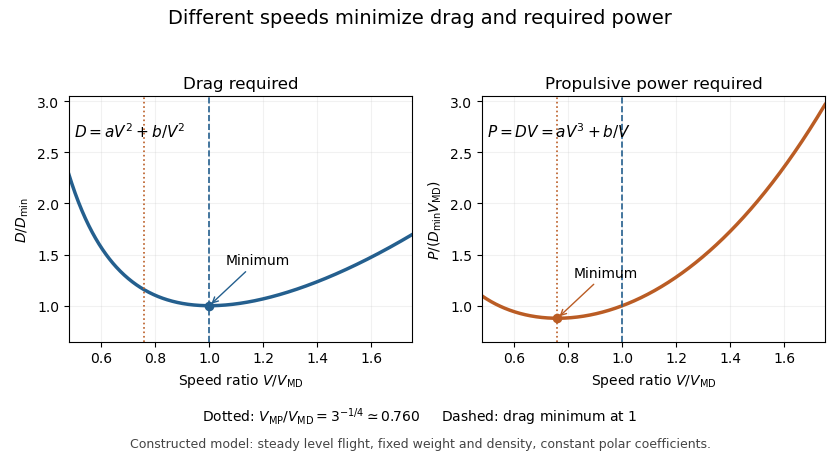
An original model uses $a=0.20$ and $b=512,000$ when $V$ is in m/s and $D$ in newtons. It gives $V_{\mathrm{MD}}=40$ m/s and $D_{\min }=640$ N, with 320 N from each term. At 30 m/s, the terms are 180 and about 568.89 N, giving a larger total of 748.89 N. The slower state nevertheless requires less mechanical power, illustrating the distinct minimum-power speed objective.

At fixed weight, minimizing drag maximizes the lift-to-drag ratio. Under a shallow, steady-glide approximation this relates to best glide through the air, whereas minimum sink speed concerns altitude loss per time. The FAA polar explicitly distinguishes the corresponding operating points.^[ref] Wind, variable coefficients or an unattainable lift coefficient can change the applicable optimum. These model results are not flight instructions or substitutes for measured aircraft performance.

The minimum-power speed $V_{\mathrm{MP}}$ minimizes the mechanical propulsive power required to sustain the specified flight state. For steady level flight with drag $D(V)$, the required power is $P(V)=D(V)V$, using speed through the air. Minimizing this product is a different problem from finding the minimum-drag speed.

With the fixed-coefficient parabolic drag polar, writeDifferentiation givesThus the stationary point is the unique global minimum for positive speed:At this point, $b/V^2=3a{V}^2$: the decreasing drag contribution is three times the increasing contribution, rather than equal to it. In lift-coefficient form, $C_L^{\mathrm{MP}}=\sqrt{3C_{D0}/k}$.

For an original numerical model with $a=0.20$ and $b=512,000$ in consistent metre-second-newton units, $V_{\mathrm{MD}}=40$ m/s and $V_{\mathrm{MP}}\simeq 30.393$ m/s. The power minimum is about 22.461 kW, with drag about 739.01 N. At the drag minimum, drag is only 640 N but power is 25.600 kW. The lower power comes from the combination of force and speed, despite the greater force.

In shallow steady unpowered descent, the gravitational energy-loss rate approximately balances $DV$, so minimizing required power relates to minimum sink speed when the same assumptions hold. This is consistent with the FAA's distinct minimum-sink and best-glide points.^[ref] A changing propulsive efficiency changes the input-power objective: if $P_{\mathrm{input}}=P/{\eta }_p(V)$, a stationary point satisfies $P^{\prime }/P={\eta }_p^{\prime }/{\eta }_p$, not generally $P^{\prime }=0$.

Attainability must also be checked. The model's optimal lift coefficient can exceed the allowed range before aerodynamic stall. The formula concerns the stated required mechanical power, not a universal minimum of fuel consumption or an operational speed recommendation.

A granulosa cell is a supporting somatic biological cell in an ovarian follicle, surrounding and interacting with the oocyte. These cells also participate in endocrine function: follicle-stimulating hormone can regulate aromatase, the enzyme converting androgen substrates such as testosterone toward estrogen production. Their behavior changes with follicular development and luteinization, so a cultured preparation is not automatically equivalent to every follicle stage.

A 2000 human-cell experiment illustrates why assay design matters. Researchers obtained granulosa-lutein cells from follicular aspirates associated with assisted reproduction. After a preincubation period, they exposed cells to follicle-stimulating hormone, washed them, and supplied testosterone for a separate two-hour test before measuring secreted estradiol. This separated the longer stimulation phase from the short aromatase activity measurement.^[ref]

The distinction is illuminating: low estradiol accumulation can reflect low enzyme activity, insufficient substrate, or changes in the preparation's responsiveness. If substrate is progressively depleted during a long culture, product accumulation alone mixes these explanations. Controlling when substrate is supplied makes the experimental question about hormone responsiveness more precise.

A theca cell is a somatic cell in the layers surrounding the granulosa cell compartment of a growing ovarian follicle. The steroid-producing thecal population responds to luteinizing hormone and supplies androgens that can become substrates for aromatase in granulosa cells. This division of biochemical work helps connect two cell populations to ovarian estrogen production.^[ref]

A 1995 experiment cultured human theca cells for four days and measured release of the androgen androstenedione. Insulin and related growth-factor treatments altered steroid output, with stronger effects in the presence of luteinizing hormone, while the tested treatments did not stimulate cell growth. The experiment separated a change in endocrine activity from a simple increase in cell number.^[ref]

An illustrative pathway therefore follows substrate rather than treating every ovarian cell as interchangeable: production of an androgen in one population can support conversion to an estrogen in another. Measuring the final product alone does not identify which upstream population changed its activity.

Feedback-informed treatment uses measured progress to inform decisions during psychological treatment. It adds an action loop to routine outcome monitoring: collect an outcome, compare the trajectory with an expected pattern, provide interpretable outcome feedback, and review what to do when progress is poor. Merely collecting scores does not test the complete feedback-and-response process.

Jaime Delgadillo and collaborators tested an outcome-feedback intervention against usual care in a cluster-randomized trial. Therapists were randomized; the analysis included 2,233 patients treated by 77 participating therapists. The intervention alerted therapists to patients at risk of a poor response and supported clinical review. Outcomes among patients treated by the same therapist therefore need to be considered within the trial's clustered design.^[ref]

Evidence for that arrangement is evidence about the tested instruments, alert rule and clinical response. It does not establish that any score dashboard, by itself, produces the same outcome. The intervention's effects must be assessed against its comparison condition and prespecified outcomes.

An orthogonal set in an inner product space is a set whose distinct vectors have zero inner product. The zero vector may be included under this definition, but every nonzero member is linearly independent of the other nonzero members. An orthonormal set additionally requires every member to have norm one.

To prove independence, suppose ${\sum }_{j=1}^m{a}_j{v}_j=0$ for distinct nonzero orthogonal vectors. With the inner product linear in the first argument, pairing with $v_k$ gives $a_k\Vert v_k{\Vert }^2=0$. Positivity of the squared norm forces $a_k=0$ for every $k$.

The standard coordinate vectors in ${\ell }^2$ form an infinite orthonormal set. Their finite linear span contains only finite-support sequences, but its closure is the whole Hilbert space. Thus completeness of an orthonormal basis refers to closed span, not to every vector being a finite linear combination. A set can be orthogonal without spanning the space.

The optimizer state is information retained by an optimization algorithm beyond the current parameter values. It can include a momentum buffer and algorithm-specific counters or running estimates. Consequently, two runs with identical parameters and current gradients can produce different next optimizer updates if their stored states differ.

For an original scalar example, minimize $f(\theta )={\theta }^2/2$ with the recurrenceThis is the momentum form with dampening, decay and the nesterov flag disabled in the PyTorch stochastic gradient descent implementation.^[ref] At ${\theta }_k=1$, $\eta =0.1$ and $\mu =0.9$, a stored $b_k=0$ gives $b_{k+1}=1$ and ${\theta }_{k+1}=0.9$. A stored $b_k=2$ instead gives $b_{k+1}=2.8$ and ${\theta }_{k+1}=0.72$. The current parameter and gradient were identical; the difference came from history.

An optimization checkpoint that saves only the parameters cannot reproduce that next step. In PyTorch, Optimizer.state_dict() stores per-parameter state and parameter-group settings such as learning rate, but not the parameter values themselves. Its parameter identifiers associate state with ordered parameter groups and are not a check of semantic parameter identity during loading.^[ref] Save and restore the corresponding parameters separately and keep the state-to-parameter association consistent. Reproducing an entire training run may additionally require the data order and other changing state.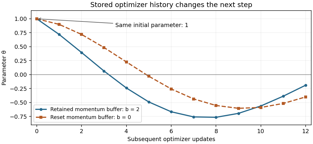

Weight decay supplies a parameter-shrinkage contribution to an optimizer update, with a coefficient commonly denoted $\lambda$. Two implementations must be distinguished. Coupled L2 regularization adds the penalty $\lambda \Vert \theta {\Vert }^2/2$ to the objective function, replacing its data gradient $g$ by $g+\lambda \theta$. Decoupled weight decay applies parameter shrinkage separately from the optimizer's processing of the data gradient. These operations are equivalent for plain gradient descent with matched coefficients, but not in general for an adaptive gradient method.^[ref]

Use the PyTorch convention here: a decoupled update shrinks parameters by $1-\eta \lambda$, where $\eta$ is the learning rate. A source writing $1-\lambda$ instead has absorbed the step-size factor into its decay coefficient. For an unmodified gradient step,In AdamW, the decay contribution does not enter the stored first- or second-moment estimates of the gradient.^[ref]

An original fixed-scaling example exposes the difference. Let $\theta =(2,2{)}^T$, $g=(1,1{)}^T$, $\eta =0.1$, $\lambda =0.2$ and diagonal matrix $A=\mathrm{diag}(1,10)$. Applying the same scaling to the entire coupled gradient givesSeparating uniform parameter shrinkage givesThe second coordinate receives different shrinkage. This is an illustrative fixed matrix, not a full AdamW simulation. With history-dependent scaling, coupling the penalty into the gradient can also alter the optimizer state. State the update equation and coefficient convention when reporting a decay setting; the label alone does not specify either.

Optical pulse temporal contrast compares a pulse's peak with weaker light at another time. For a radiant power trace with peak $P_{\max }>0$, explicitly choose either the peak-to-local ratio $C(t)=P_{\max }/P(t)$ or its inverse $r(t)=P(t)/P_{\max }$. The first is at least one where the local power is positive; the second lies between zero and one. With a fixed transverse beam shape, the same ratio can be formed from light intensity. If the beam shape changes with time, specify the spatial sampling instead of identifying local intensity and total power.

A plateau at $10^{-3}$ of the peak has $r=10^{-3}$ and $C=1000$. Expressing this power ratio as optical contrast in decibels givesFor an amplitude ratio $A$ whose power ratio is $A^2$, the same definition gives $10{\log }_{10}(A^2)=20{\log }_{10}A$. Contrast also needs a delay or time range: an optical prepulse, an optical postpulse and a long optical pulse pedestal can have the same relative height but different positions and laser pulse energies. The pedestal energy fraction additionally requires integration over the contribution's duration.

A useful nonlinear measurement is third-order intensity autocorrelation. In an ideal instantaneous model, an input light intensity $I(t)$ generates a second-harmonic gate proportional to $I^2(t)$. Sum-frequency generation with a delayed fundamental replica gives a recorded signal proportional toThe instrument measures this cross-correlation, rather than simply reading $I(\tau )$. Finite gate width, phase matching, spatial overlap and detector response enter the interpretation.

The1998/99 instrument of J. Collier and colleagues used second-harmonic generation, a Wollaston prism and an optical biprism to form crossing fundamental and harmonic beams. A second crystal generated the sum-frequency signal, imaged through optical filters onto a charge-coupled device. Position encoded delay. An inserted glass etalon produced a delayed replica near $1.5\times 10^{-3}$ of the main signal, recorded on one side of the correlation peak. Figure4 combines window settings shifted with etalons.^[ref]

An independent ideal calculation explains both the asymmetry and a possible third-order pulse correlation ghost. Let $I(t)=g(t)+\epsilon g(t-d)$ represent two identical-shape pulses with well-separated supports and correlation lobes, with the second weaker and delayed. Squaring introduces no overlap term. If $A_g(\tau )=\int g^2(t)g(t+\tau )dt$, expansion givesThe delayed replica produces a lobe of relative order $\epsilon$, while the opposite-delay ghost has order ${\epsilon }^2$. For $\epsilon =0.01$, the scales are about $10^{-2}$ and $10^{-4}$ respectively. These values are predictions of the stated ideal model. Assigning every small correlation feature directly to a separate input pulse would miss this distinction.

A nondetection below the measurement floor establishes a bound under a detection model, rather than demonstrating that no light exists there. Finite dynamic range, detector baseline subtraction, delay coverage and resolution should accompany a reported contrast trace. The Sequoia manufacturer likewise distinguishes optical temporal resolution from the scan step; making that step smaller does not alone narrow the optical response.^[ref]

The pedestal energy fraction is the fraction of an optical pulse's laser pulse energy assigned to its optical pulse pedestal. Specify the decomposition and integration interval before quoting it. For a nonnegative additive radiant power model $P(t)=P_m(t)+P_p(t)$,The assumptions $0\le P_p\le P$ imply $0\le f_p\le 1$ by integration. A pedestal fit is a model of the measured radiant power; it is not automatically a unique physical separation into optical fields. Overlapping fields with optical coherence can have wave interference terms, so their separate field energies cannot generally be added as though those terms were absent.

The distinction from optical pulse temporal contrast is quantitative. Use the stipulated rectangular model of optical pulse pedestal: a main contribution has height $P_0$ and duration $\tau$, while a centered pedestal has height $\alpha P_0$ and duration $T\ge \tau$. For $0<\alpha <1$, the total peak is $(1+\alpha )P_0$ and the power full width at half maximum remains $\tau$. Define peak-to-pedestal contrast $C=(1+\alpha )/\alpha$. ThenHalf the laser pulse energy is in the modeled pedestal when $T=(C-1)\tau$. A large peak-to-pedestal ratio therefore does not by itself imply a small energy contribution.

For an original comparison, fix $C=1001$ and the same $P_0,\tau$ in both traces. With $T=10\tau$, the pedestal fraction is $10/1010\approx 0.00990$; with $T=1000\tau$, it is $1/2$. Thus the same contrast and power FWHM can coexist with about1% or50% pedestal energy. At fixed finite $C$, increasing the pedestal duration can make $f_p$ approach one without changing that FWHM.

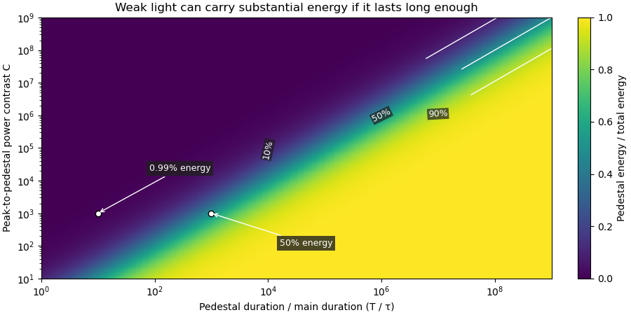
Optical energy outside a time gate is a related observable that avoids assigning a pedestal underneath the main peak. For a specified gate $G$ containing that peak,In the rectangular example with $G$ equal to the main interval, $f_{\mathrm{out}}=\alpha (T-\tau )/(\tau +\alpha T)$. At $\alpha =10^{-3}$ and $T=1000\tau$, this is $0.4995$, while $f_p=0.5000$. The difference is pedestal power inside the gate, which the outside-gate measurement does not label separately.

The analysis must also specify its temporal coverage and detector baseline subtraction. Subtracting actual weak light as though it were detector background changes the inferred laser pulse energy. A short detection time gate omits outlying light instead. Neither operation is justified solely by knowing the peak-to-pedestal contrast. The Sequoia technical sheet illustrates why temporal coverage and resolving power are separate instrument properties: it lists scan range, scan resolution and optical temporal resolution independently.^[ref]

An etalon round-trip delay is the extra envelope travel time associated with one additional internal round trip in an etalon. At normal incidence, for a transparent plate of thickness $L$ and a sufficiently narrowband optical pulse,The relevant quantity is group refractive index, since the delay concerns the pulse envelope. The extra propagation phase is $\varphi (\omega )=2\omega n(\omega )L/c$; its derivative gives $d\varphi /d\omega ={\tau }_{\mathrm{rt}}$. This assumes negligible frequency-dependent reflection phase and treats dispersion locally.

For an original chosen plate with $L=3.0\mathrm{mm}$ and $n_g=1.60$, the delay is about $32.0\mathrm{ps}$. A pulse transmitted after one extra round trip appears that much later than the directly transmitted pulse. Another extra round trip adds the same delay in this local model, producing an echo sequence. The optical postpulse article separately describes the reflection losses that determine echo energies.

The frequency-domain connection gives an independent consistency check. Neighboring transmission resonances differ in round-trip phase by $2\pi$, so the local free spectral range satisfiesThe example predicts about $31.2\mathrm{GHz}$. This etalon delay inferred from free spectral range uses the same local dispersion assumptions; the spacing can vary across a broad spectrum.

The historical third-order correlator calibrated its delay coordinate by inserting a BK7 etalon of known thickness into an arm and measuring the trace shift.^[ref] A plate inserted into an arm also changes the direct propagation delay relative to the displaced air path; that single-pass insertion delay is distinct from the echo's extra internal round trip. Oblique incidence, dispersive coatings and broad-band pulse reshaping require a more complete propagation model.

Baseline-trajectory dependence of local respiratory time constants means that the linearized response can change as volumetric flow rate and elastic state change during a breath. A time constant measured at one operating point need not describe the entire trajectory, even when the underlying constitutive laws stay fixed.

In an original one-compartment model, let pressure satisfy $P=G(v)+F(\dot{v})$. Around a specified baseline $v_0(t)$, a small perturbation obeysThe frozen-coefficient local time constant is $\tau (t)=R(t)/E(t)$ when both coefficients are positive. For zero perturbing drive, the actual response is insteadThis follows by an integrating factor for the linear differential equation. The accumulated relaxation rate, rather than one selected endpoint value, controls the decay.

Choose a stipulated driven baseline volumetric flow rate $Q_0(t)=0.5e^{-t/t_b}$ L/s with $t_b=1$ s. Let elastic compliance be 0.20 L per cm water and resistive pressure be $F(Q)=2Q+4Q|Q|$ in the corresponding numerical units. Then $E=5$ and $R(t)=2+4e^{-t/t_b}$. The local time constant decreases from 1.2 s toward 0.4 s as the baseline volumetric flow rate falls.

Writing numerical time $u=t/t_b$, the homogeneous perturbation has the exact relative amplitudeAt one second it is about 0.322. Freezing the initial time constant would instead give $e^{-1/1.2}\approx 0.435$; freezing the limiting value would give $e^{-1/0.4}\approx 0.082$. These are distinct approximations to a changing-coefficient problem, not measured patient responses.

The baseline here is explicitly driven: its external pressure must sustain the chosen trajectory. It is not claimed to be the natural unforced expiration law of the nonlinear compartment. The primary respiratory pilot study compares methods that depend on volumetric flow rate, pressure and expiratory time scales, and discusses why expiration need not have one exponential time constant.^[ref] A local fitted value belongs to its operating trajectory and observation interval.

A good cover is an open cover in which every nonempty finite intersection of covering sets is contractible. In particular, each individual covering set must be contractible. Requiring only contractible sets, without their intersections, is weaker.

For example, two long arcs can cover a circle while their overlap consists of two separated arcs; this is not a good cover. Three suitably chosen shorter arcs cover the circle with pairwise interval overlaps and no triple overlap. That is a good cover whose nerve is a triangle boundary.

The nerve records a simplex for each nonempty finite intersection. For a smooth manifold with an open good cover, the nerve lemma identifies the homotopy type of the nerve with that of the manifold. Contractible intersections therefore permit local data to encode global topology combinatorially. Empty intersections contribute no simplex and impose no contractibility requirement.