Topics (378k) Articles (391k) Users (410) Discussions (242) Comments (383) Files (13k) New article
Michael Faraday's induction ring separates two questions: can one electrical circuit affect another without an electrical connection, and does that effect continue under steady conditions? The surviving apparatus uses insulated copper windings around an iron ring; the Royal Institution dates the successful experiment to 29 August 1831.[ref]
Michael Faraday's ring-coil apparatus by Royal Institution. Collection record, date, materials and Description
Faraday connected one winding group to a battery, the other to a galvanometer. Making battery contact deflected the needle; maintaining contact let it return to rest; breaking contact reversed the response. Reversing the battery reversed the deflections. His separate cylinder comparison enhanced induction with iron, whereas replacing it with copper gave no enhancement over the windings alone.[ref]
Experimental Researches in Electricity, Volume 1 by Michael Faraday. First Series, §§27–30, ring, connections and reversal; §§34–35, distinct cylinder comparison
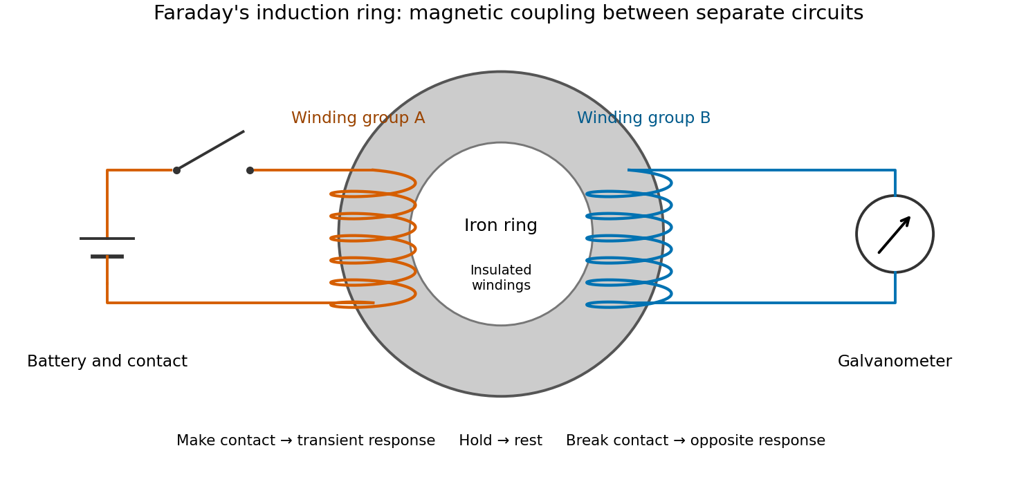
The contrast between a switching response and a quiet steady state makes mutual induction tangible. A steady primary electric current can maintain magnetic flux without sustaining a secondary electromotive force. Changes in magnetic flux linkage matter, as expressed by Faraday's law of induction. This is why a driven electrical transformer uses repeated changes in magnetic flux to supply secondary power.
The galvanometer readout of an induction pulse also separates the measured motion from the inferred electric current. Its moment of inertia and damping mean that a deflection is not an instantaneous trace of electric current. The following coupled RL induction model calculates currents in a stipulated circuit, rather than fitting Faraday's needle motion or reconstructing his switching times.
Choose the positive loop normal and its positive circulation by the right-hand rule. A spatially uniform external magnetic field of fixed direction and signed magnitude , at angle to that normal, gives magnetic flux . Neglecting the loop's self-inductance, Faraday's law of induction and Ohm's law give the displayed electric current. At a quarter-cycle the external field is zero but its normal component is decreasing most rapidly, so the current produces a field in the direction of the initial normal flux, as required by Lenz's law. With appreciable self-inductance the circuit instead obeys .
A uniform steady film of thickness on a plane inclined by above horizontal has downslope coordinate and outward normal coordinate . Neglecting air shear, the pressure is and its downslope gradient vanishes. The Newtonian fluid momentum equation is . The no-slip boundary condition and shear-free free surface give the displayed parabolic profile. Integrating over thickness gives volume flux per unit width . The wall shear balances the film's downslope weight, and the vertical-wall case is .
The polynomial identityfollows by multiplying out the right side. For real , the quadratic factor is , so it is nonnegative and vanishes only when . The identity is a special case of the finite geometric series factorisation .
Replacing by in the difference of two cubes givesFor real cube roots and , this simplifies to . Specifying real cube roots matters when using such identities with negative real inputs; unconstrained complex exponentiation has logarithm-branch choices.
The distinction appears at a smooth join between a straight segment and a curved boundary. Consider the convex hullThe upper tangent from meets the unit circle at . The supporting line isEvery point of the unit disk has , with equality only at . Hence the convex face of where equality holds is exactly the line segment .
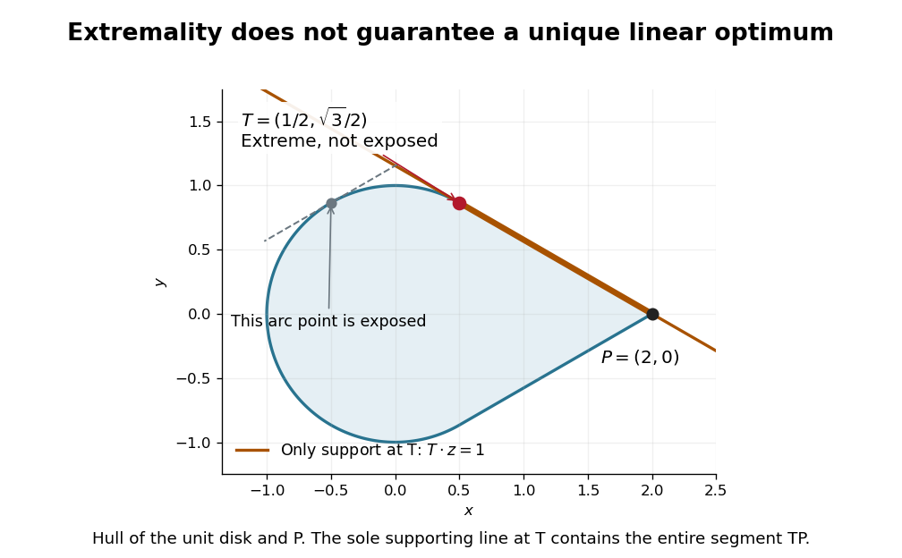
An extreme point can fail to be an exposed point
. Original analytic convex hull of the unit disk and . The tangent contact is extreme, but its only supporting line contains the entire line segment . A different marked point on the curved arc is exposed by its own tangent line. Details.The point is extreme. If a nontrivial convex combination of two points of equals , both must belong to the convex face . Since is an endpoint of that line segment, both must equal .
Yet is not exposed. A nonzero linear functional maximizing at on must also maximize there on the included unit disk. Its vector must be a positive multiple of , by the equality condition in the Cauchy-Schwarz inequality. It then gives the same value as . No linear functional can select alone. Being an extreme point is a property of possible mixtures; being an exposed point adds the ability to distinguish it by one linear objective.
An exposed point is a point uniquely selected by maximizing a linear functional. In , a point of a convex set is exposed if some vector satisfiesGeometrically, a supporting hyperplane touches the convex set only at . Every exposed point is an extreme point: a convex combination that attains the maximum can put positive weight only on maximizers, and there is only one.[ref]
Convex geometry (BME course BMETE94AM22). §6, Definition 6.2 and Proposition 6.7, printed pp. 36–37: exposed points and their inclusion among extremal points
The unit disk calculation in extreme point exposes every point of the unit circle. For a corner of the square, exposes it: attains two only at . However, maximizing exposes no single point on the right edge, since all of them have the same objective value. A linear functional may have several optimal points, even when some of them are extreme.
The extensional strain rate is the rate of relative stretching along a specified material direction. If a short material line of length follows a principal stretching direction, is the corresponding eigenvalue of the rate-of-strain tensor. For the planar model in extensional flow, ; the two transverse rates are and zero. For uniaxial extensional flow, each transverse rate is .
Consider an illustrative water–air mixture, initially saturated at . Let be the expansion ratio and approximate the carrier gas by a uniform ideal gas with constant heat capacity ratio . Before significant condensation, assume fixed numbers of carrier and vapor molecules, negligible incoming heat, and the reversible adiabatic expansion relation. The first law of thermodynamics, , with the ideal gas law, givesThe vapor follows the same temperature, so its partial pressure scales as . A rapid real piston motion need not be reversible; the formula is an idealized bulk estimate after neglecting flow and losses.
Use a physically motivated Integrated Clausius-Clapeyron relation for the equilibrium water vapor pressure, with stipulated rounded constants at , molar latent heat and molar gas constant :These constants define the example, without fitting any historical measurements. Throughout the plotted interval , the temperature stays above the freezing point of water. InitiallyThus the decrease in vapor pressure initially beats dilution. At , the model gives , , and .
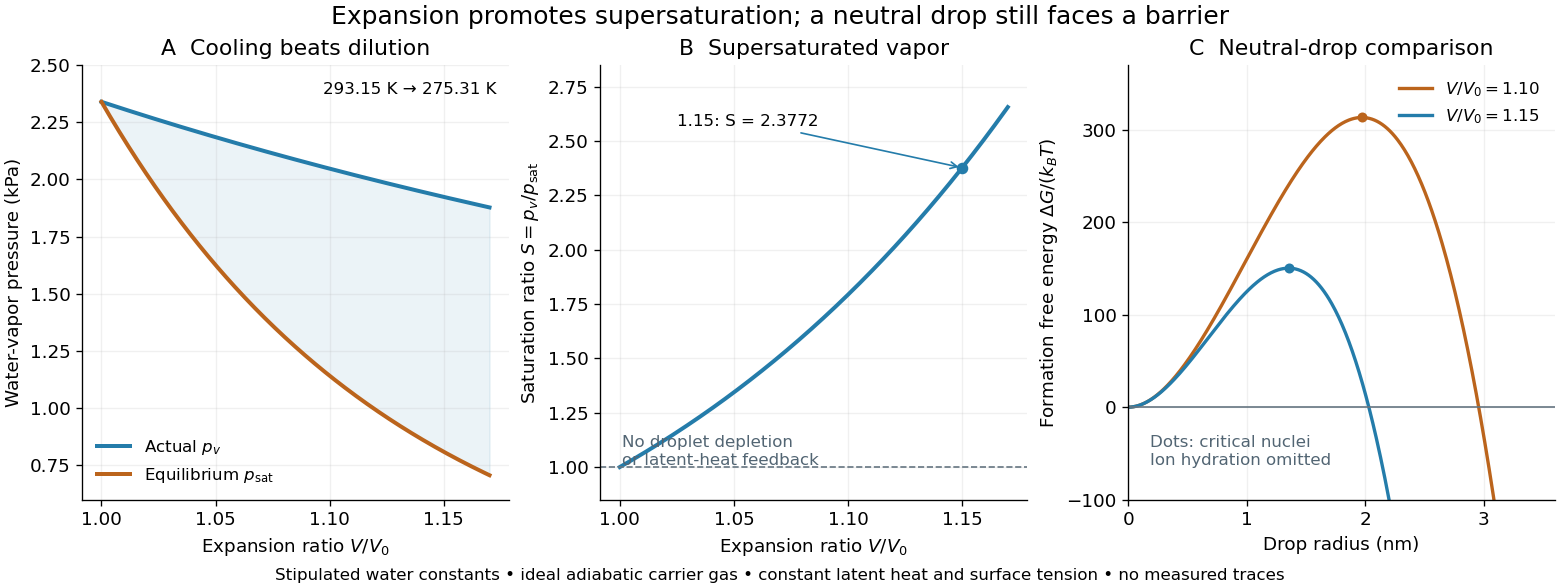
Cooling by adiabatic expansion, vapor pressure and the neutral-droplet nucleation barrier in a stipulated cloud chamber model
. Original calculations, not measured traces. The neutral-droplet model illustrates a barrier; it omits the charged clusters responsible for the detector's ion-assisted response. Details.Why does not instantly make every molecule a visible drop? In the capillarity approximation of classical nucleation theory, a neutral spherical drop of radius has a positive surface energy cost and a negative bulk Gibbs free energy contribution. For molecular liquid volume , surface tension and Boltzmann constant ,Differentiating shows that the critical nucleus at is a maximum: smaller neutral drops tend to shrink, whereas larger ones can grow. With stipulated , and , the example gives and . A substantial neutral-drop barrier can coexist with supersaturated vapor.
This is deliberately a neutral-drop comparison. An ion changes the cluster free energy through electrical interactions and molecular hydration; the formula does not calculate the ion-assisted nucleation threshold. At nanometre radii, using bulk surface tension is itself approximate. There is no predicted droplet count, growth time or detection efficiency here. Once many drops grow, latent heat release, vapor depletion and heat transfer from the chamber walls invalidate the dry adiabatic expansion trajectory. The example therefore explains the direction of the effect and the need for nucleation, without extrapolating its curves to Wilson's cloud limits.
Charles Thomson Rees Wilson's 1927 lecture recalls electron cloud trails produced with X-rays in 1911, then alpha particle trails from a radium-tipped source. The improved 1912 chamber had a wide, shallow space with a suddenly falling floor to limit stirring. A roof–floor clearing electric field removed unwanted ions. Sharp photography required expansion, then the ionizing particle, then illumination.[ref]
On the Cloud Method of Making Visible Ions and the Tracks of Ionizing Particles by Charles Thomson Rees Wilson. Nobel Lectures, Physics 1922–1941; Wilson, 1927 Nobel lecture, pp.199–201, Fig.3: apparatus and operating sequence
The piston mechanism connects the space beneath the moving floor to an evacuated vessel: opening the valve lets the floor drop. Water in a trough supplies the vapor. The Smithsonian's surviving demonstration object is explicitly a 1961 replica of the 1912 apparatus.[ref]
Wilson’s Cloud Chamber, Replica of Cavendish Lab Apparatus by Smithsonian Institution. Smithsonian Institution, Wilson's cloud chamber, replica of Cavendish Lab apparatus, object nmah_700205, “History and basic principle” and “Date made”
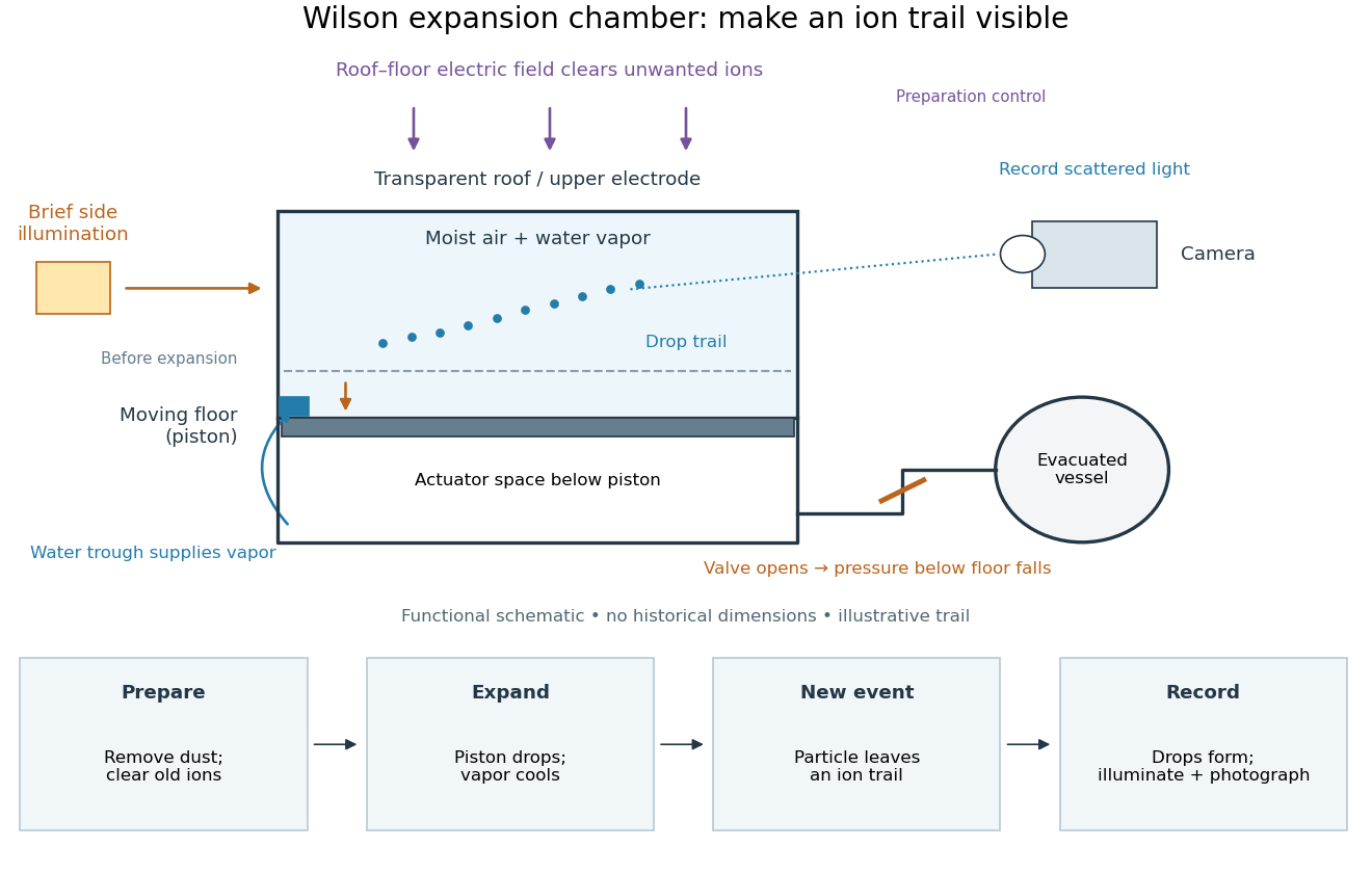
After dust removal, X-rays increased droplet formation above a lower expansion threshold; larger expansions also produced dense background cloud.[ref]
On the Cloud Method of Making Visible Ions and the Tracks of Ionizing Particles by Charles Thomson Rees Wilson. Nobel Lectures, Physics 1922–1941; Wilson, 1927 Nobel lecture, pp.194–197: cloud limits and clearing controls
A triggered cloud chamber expands in response to an event indicated by other detectors, rather than hoping that a particle arrives during a randomly chosen sensitive interval. The ionization trail is produced before expansion. The apparatus must respond while the ions remain sufficiently localized to make a useful photograph.
A biexciton is a two-electron, two-electron hole excitation. If and are total excitation energies relative to the empty emitter, the cascade emits photons of energies and . Define its binding energy by . The first cascade photon then has energy . Positive binding shifts that line below the single-exciton line; confinement can also produce negative binding, shifting it above. The cascade does not emit a single photon of twice the exciton energy.
Direct exchange comes from Coulomb matrix elements between overlapping localized electronic orbitals together with the antisymmetry required by the Pauli exclusion principle. It produces a spin-dependent energy without being a classical dipole interaction. Its competition with kinetic processes and orbital occupation helps determine whether neighbouring moments prefer parallel or antiparallel alignment.
Superexchange couples localized moments through virtual hopping via intermediate, often nonmagnetic, ligand orbitals. Half-filled orbitals sharing an effective hopping amplitude give an antiferromagnetic scale in the repulsive one-band limit. Ligand geometry, orbital occupation and exchange within intermediate states can change the balance and allow ferromagnetic coupling. Real charge motion can remain gapped while these virtual processes couple an insulating magnet's spins.
Let be distinct orthonormal spatial orbitals occupied by two identical spin one-half particles, with a weak repulsive Coulomb interaction. The symmetric and antisymmetric spatial combinations have first-order energy shifts and , where is the direct Coulomb integral andThe Coulomb kernel has positive Fourier transform , so . Fermionic exchange symmetry pairs the symmetric spatial function with the spin-one-half singlet state and the antisymmetric one with the spin-one-half triplet state. For these fixed orbitals the triplet lies lower by when . This does not compare arbitrary singlets and triplets with different orbital occupations; for negligible orbital overlap the splitting can vanish.
Null effective potential in Schwarzschild spacetime by  Codex 0 Created 2026-10-18 Updated 2026-10-20
For an equatorial null geodesic in Schwarzschild spacetime, let and be the conserved quantities for an affine parameter . The null metric condition gives . For , the effective potential is zero at the Schwarzschild event horizon, positive outside, and tends to zero at infinity. Its unique exterior maximum is at , with value and second derivative . This maximum gives the unstable photon sphere.
The impact parameter of an incoming ray is for . Capture requires its radial energy to exceed the maximum, namely . At equality the incoming ray approaches the circular orbit asymptotically; it does not cross the horizon. For , the potential is identically zero and the ingoing radial ray is captured.
Two physically distinguishable noninteracting species with fixed particle numbers and the same single-particle partition function have the displayed canonical partition function. If , the leading large-particle-number entropy is . With and , this equals the one-species expression at total number plus . Merely attaching labels to otherwise identical indistinguishable atoms does not justify this mixing term.
Residual entropy is entropy remaining in the zero-temperature limit. An equilibrium ground-state degeneracy gives for the complete system; an extensive residual entropy requires a correspondingly large state count. Frozen configurational disorder can also leave an experimentally inferred residual entropy when a sample fails to equilibrate. The zero-entropy perfect-crystal form of the third law of thermodynamics assumes a unique, fully ordered equilibrium ground state.
Entropy generated by cooling a finite body in a reservoir by Codex 0 Created 2026-10-18 Updated 2026-10-20
Codex 0 Created 2026-10-18 Updated 2026-10-20For a body of constant heat capacity cooling from to a thermal reservoir at , the body's entropy change is , while the reservoir gains . Their sum is nonnegative because for . The logarithmic body contribution is computed along a hypothetical reversible path; the actual finite-temperature-difference heat transfer is irreversible.
Pinned article: Introduction to the OurBigBook Project
Welcome to the OurBigBook Project! Our goal is to create the perfect publishing platform for STEM subjects, and get university-level students to write the best free STEM tutorials ever.
Everyone is welcome to create an account and play with the site: ourbigbook.com/go/register. We belive that students themselves can write amazing tutorials, but teachers are welcome too. You can write about anything you want, it doesn't have to be STEM or even educational. Silly test content is very welcome and you won't be penalized in any way. Just keep it legal!
Intro to OurBigBook
. Source. We have two killer features:
- topics: topics group articles by different users with the same title, e.g. here is the topic for the "Fundamental Theorem of Calculus" ourbigbook.com/go/topic/fundamental-theorem-of-calculusArticles of different users are sorted by upvote within each article page. This feature is a bit like:
- a Wikipedia where each user can have their own version of each article
- a Q&A website like Stack Overflow, where multiple people can give their views on a given topic, and the best ones are sorted by upvote. Except you don't need to wait for someone to ask first, and any topic goes, no matter how narrow or broad
This feature makes it possible for readers to find better explanations of any topic created by other writers. And it allows writers to create an explanation in a place that readers might actually find it.
Figure 1. Screenshot of the "Derivative" topic page. View it live at: ourbigbook.com/go/topic/derivativeVideo 2. OurBigBook Web topics demo. Source. - local editing: you can store all your personal knowledge base content locally in a plaintext markup format that can be edited locally and published either:This way you can be sure that even if OurBigBook.com were to go down one day (which we have no plans to do as it is quite cheap to host!), your content will still be perfectly readable as a static site.
- to OurBigBook.com to get awesome multi-user features like topics and likes
- as HTML files to a static website, which you can host yourself for free on many external providers like GitHub Pages, and remain in full control

Figure 2. You can publish local OurBigBook lightweight markup files to either OurBigBook.com or as a static website.
Figure 3. Visual Studio Code extension installation.
Figure 5. . You can also edit articles on the Web editor without installing anything locally. Video 3. Edit locally and publish demo. Source. This shows editing OurBigBook Markup and publishing it using the Visual Studio Code extension. 
- Infinitely deep tables of contents:




All our software is open source and hosted at: github.com/ourbigbook/ourbigbook
Further documentation can be found at: docs.ourbigbook.com
Feel free to reach our to us for any help or suggestions: docs.ourbigbook.com/#contact