Topics (384k) Articles (398k) Users (410) Discussions (242) Comments (383) Files (13k) New article
Past exam of the advanced quantum physics course of the University of Cambridge 2017 3 Solution by  Codex 0 Created 2026-10-18 Updated 2026-10-20
The Zeeman effect comes from . For an electron, the orbital and spin magnetic moments are approximately and , respectively. This explains both the sign and the relative factor two in the term linear in . The second term is the spin-orbit interaction: the electron's motion through the atomic electric field produces a magnetic interaction in its rest frame. The relativistic correction, including Thomas precession, and the radial expectation value are incorporated into . This effective Hamiltonian retains the linear Zeeman splitting and spin-orbit coupling, while omitting diamagnetic and hyperfine structure corrections.
Define the angular momentum ladder operators by and similarly for . Direct expansion givesso adding gives the required scalar product. The off-diagonal terms change and in opposite directions. Consequently commutes with , and remains a good quantum number at every magnetic field.
In the given product eigenbasis, the diagonal matrix elements areFor and , the only off-diagonal couplings are between and , and between and . Each relevant orbital ladder factor is and each spin ladder factor is . Multiplying by gives . ThereforeAll other off-diagonal entries vanish either by the ladder endpoints or by conservation of . This derives every entry of the displayed matrix.
The stretched states have no mixing and yieldThe block is , while the block is . Taking the trace and determinant of each block gives the remaining four energy eigenvalues:The subscripts indicate and the superscripts indicate the upper or lower root. These formulas are the Zeeman spectrum for orbital angular momentum one and remain valid for either sign of .
For the usual ordering , including sodium, the zero-field states follow fromThe quartet lies at and the doublet at , separated by . In a weak magnetic field, the Landé g-factors giveThese label the curves near . In a strong magnetic field, the Paschen-Back effect makes the appropriate approximate labels:for the mixed states, with the stretched-state formulas already exact. The branch connections for areWithin a fixed , the nonzero coupling prevents a crossing; this is an avoided crossing. Curves with different may cross because the Hamiltonian does not couple them.
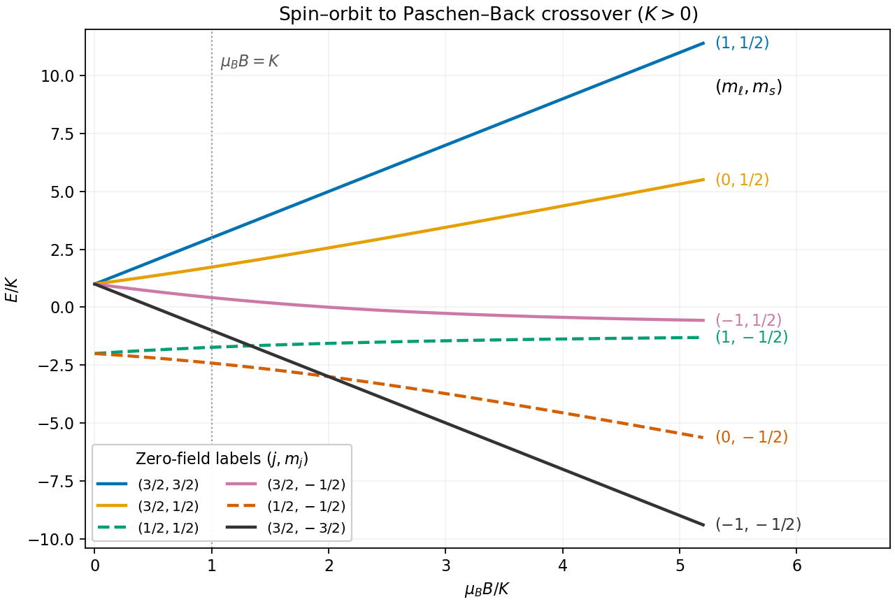
Exact spin-orbit and Zeeman energies for orbital angular momentum one and positive spin-orbit constant
. Details. For the sodium estimate, the zero-field frequency separation fixesThe lower doublet has shifts . The Sodium D-line Zeeman pattern gives photon-frequency shifts times for D and for D. Thus the highest-frequency D component and lowest-frequency D component approach each other by . Extrapolating the weak-field Zeeman splitting givesso the crossover occurs at a field of order , where and the weak-field approximation is becoming marginal.
The exact eigenvalues refine the estimate within this Hamiltonian. The relevant photon energies, with a common zero-field reference omitted, are and . The corresponding electric dipole transitions have and , respectively. Equating them givesIts positive solution is , hencein the retained model. The crossing is between optical transition frequencies; the participating upper states themselves need not be degenerate.
A quasihole adds one zero at per electron; its local deficit carries positive electric charge .[ref]
Anomalous Quantum Hall Effect: An Incompressible Quantum Fluid with Fractionally Charged Excitations by Robert Laughlin. pp. 1396–1397, Eqs. (13), (15) and screening argument
Here is a transport counting outline, conditional on an incompressible quantum Hall fluid. Inserting one magnetic flux quantum slowly compared with , where is the excitation energy gap, produces a circulating electric field by Faraday's law. The transverse sheet conductivity sends a radial electric current whose time integral has magnitudeThe opposite electric charge moves to the boundary, so the total electric charge remains conserved. The counted deficit belongs to a collective quasiparticle; no individual electron has been cut into pieces. The argument assumes the gapped fluid and its Hall response, and is not a consequence of the finite two-electron normalization integral.
Consider the original two-electron example obtained by taking in the Laughlin wavefunction, with no additional polynomial for the centre of mass. Introduce , relative complex coordinate , separation , and dimensionless separation . Since , the probability density factorizes:Integrating out leaves an isotropic relative probability density. Define per unit dimensionless area and per unit dimensionless separation:The physical areal probability density is . The probability of a separation between and is . The extra comes from the Jacobian determinant in polar coordinates: a thin annulus has area . Omitting that factor changes the question being answered.
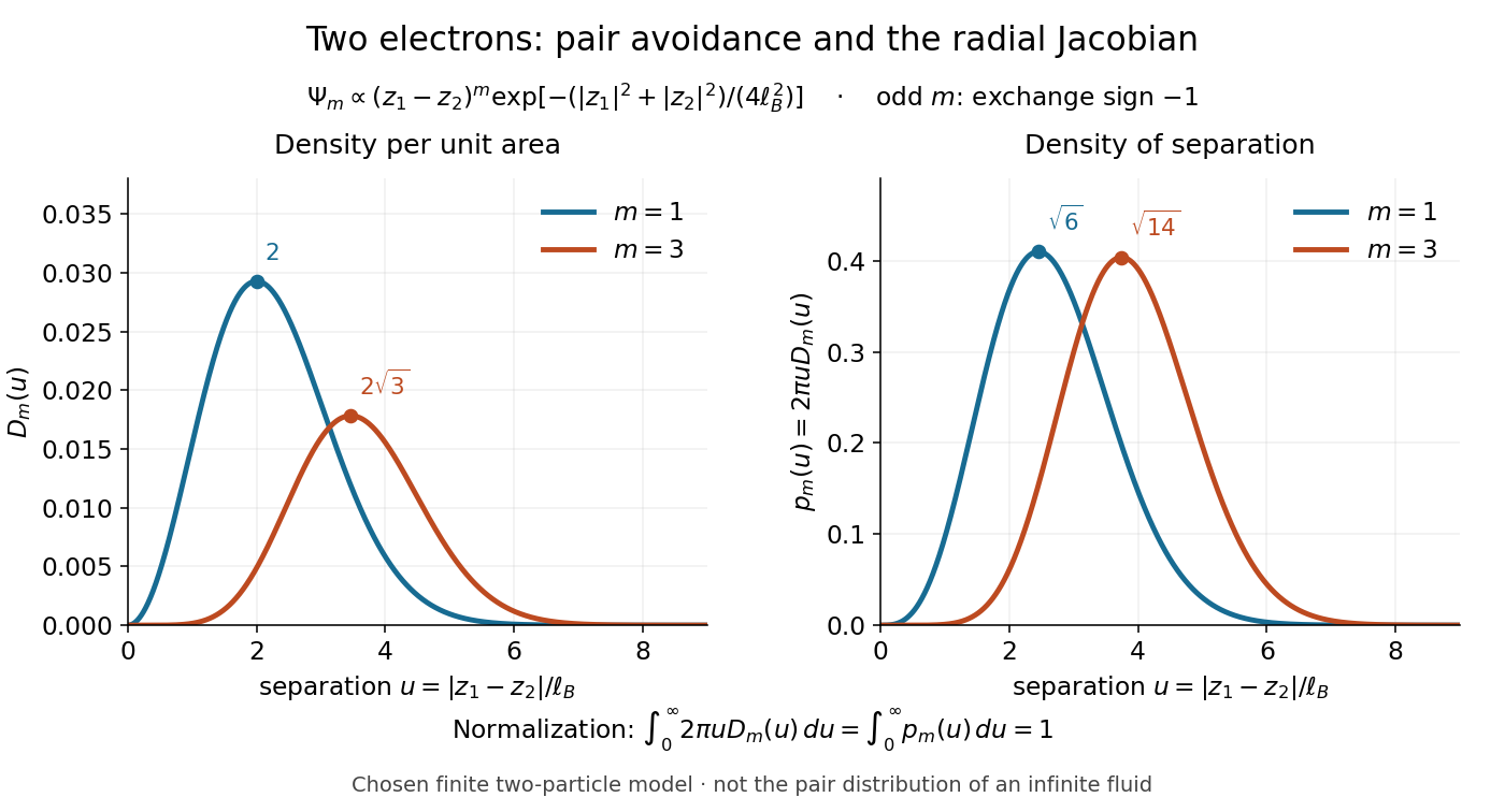
Both wavefunction normalization and the peak shift can be checked exactly. The substitution gives the Gamma function integralFor , logarithmic differentiation givesConsequently the areal maximum lies at , while the most probable separation lies farther out, at . For these are and ; for , and . The same substitution gives , so the root mean square separations are and respectively. The distinction between a probability density maximum and a radial maximum therefore has a directly calculable geometric origin.
This two-electron model explains exchange and pair avoidance. It does not establish a nonzero many-particle spectral gap, an extended quantum Hall plateau, or the topological properties of a fluid in the thermodynamic limit. Those require additional many-electron reasoning and experimental tests.
Define the amplitude evanescent penetration depth as the distance at which the electric field wave amplitude falls to of its surface value:The squared-field envelope decays twice as fast:The same normalized exponential decay describes the tangential average Poynting vector for the TE polarization above. An intensity penetration depth convention often means ; it must not be confused with amplitude depth or interpreted as outgoing normal light intensity.
For the stipulated , , and ,At the normalized wave amplitude is approximately , and its squared envelope is approximately . At , these become and , respectively. The quantity inside the square root is dimensionless, so has inverse-length units and both depths have length units.
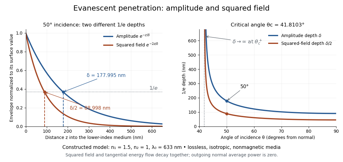
Constructed evanescent-field model at 633 nm: amplitude and squared-field decay at 50 degrees, and their penetration depths as incidence increases above the critical angle
. Details. The sharp angular dependence has a simple explanation. For with small and measured in radians, a first-order Taylor expansion givesThus as : exponential confinement disappears continuously. With fixed refractive indices, decreases as the angle of incidence increases and approaches as . This is a limit of the normalized depth; exactly grazing incidence supplies zero incident normal power. Real beam widths, angular spreads and optical dispersion matter when applying these ideal plane electromagnetic wave predictions near the threshold.
A doped semiconductor at frequencies far below its bound-electron resonances can haveFor a weakly absorbing nonmagnetic half-space adjacent to vacuum, the normal-incidence optical reflectance is minimized near refractive-index matching, . When and is small this gives . The zero of the real part of , near , is a distinct frequency. Increasing the carrier density shifts the minimum to shorter wavelength if the carrier effective mass and background response remain fixed. With appreciable loss, the minimum must be found from the full complex Fresnel equations.
Fill the lower energy band of the dimerized tight-binding chain with both spin states. Take zero on-site energy and measure ground-state energy per doubled primitive unit cell. State counting in a Bloch band and giveEquivalently, for , , where is the complete elliptic integral of the second kind in the modulus convention.
For fixed and , the change isThe logarithm comes from states near the edge of the Brillouin zone. Put . To leading order the square root there is . For a fixed small cutoff , direct integration givesThe rest of the band, and the higher-order corrections near its edge, contribute only ; multiplying by gives the displayed asymptotic expansion. Here the remainder uses Big O notation. The negative logarithmic term exceeds any fixed quadratic elastic cost , , for sufficiently small nonzero . This explains the zero-temperature instability to a Peierls distortion in the ideal chain model.
Exclusion and the energy of two electrons in three spatial levels by Codex 0 Created 2026-10-18 Updated 2026-10-20
Codex 0 Created 2026-10-18 Updated 2026-10-20Consider an original noninteracting model with three orthonormal spatial orbitals at energies , where . Both spin projections are available at each energy, so there are six spin orbitals. The Quantum Hamiltonian is , with no interaction between particles and no dependence on spin. Comparing its allowed ground states isolates the effect of fermionic exchange symmetry.
For two distinguishable spin-one-half particles, the spatial ground state is and any of four independent two-spin states is possible: and ground-state degeneracy four. For two identical electrons, both can still occupy , using and , but there is just one allowed ground state: the symmetric spatial factor times the spin-one-half singlet state,Exclusion has reduced the ground-state degeneracy without raising the ground state energy.
Now restrict both particles to the same spin projection . Distinguishable particles can still both occupy , so . Identical electrons must occupy different spatial orbitals; the lowest choice is , withThe spin factor is a spin-one-half triplet state, and the spatial factor is antisymmetric. These are ground states within the restricted parallel-spin sector, not the unrestricted two-electron ground state. Both restricted models have ground-state degeneracy one.
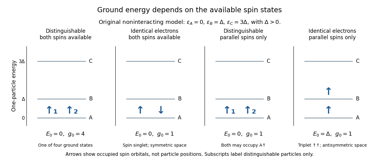
The first excited two-electron energy in the unrestricted model is , with four independent quantum states: one occupant in , one in , and two spin choices for each. A basis adapted to particle exchange operators separates these into one spin-one-half singlet state with symmetric spatial factor and three spin-one-half triplet states with antisymmetric spatial factor. All four have equal energy in this model. Singlet versus triplet does not by itself determine an energy gap; an interaction or a spin-dependent term is needed to split them.
As a further count, the full two-electron space has dimension . Its energies in units of and corresponding multiplicities are and . For distinguishable spin-one-half particles the ordered tensor product instead has dimension , with multiplicities at those same energies. These are exact model counts, not atomic measurements. The higher restricted ground state energy follows from removing forbidden quantum states; the Quantum Hamiltonian contains no additional “exclusion force”.
For the interaction built from the total two-electron spin and orbital angular momentum, set . The spin-dot-product eigenvalue identity then gives the shift in the title. In the first excited two-electron oscillator manifold, the singlet has and zero shift with multiplicity three. The triplet has , with shifts and multiplicities .
The multiplicities sum to twelve, and their weighted shift sums to zero. The specified interaction preserves both and ; it is distinct from summing separate single-electron spin-orbit interactions. Its shifts are exact within this model's invariant oscillator manifold, with weak coupling ensuring the original level ordering remains useful.
Frustrated total internal reflection occurs when a nearby second high-index dielectric couples to the evanescent field in total internal reflection, allowing power to cross a finite low-index gap. The extra boundary changes the dielectric-interface boundary conditions; the gap field need not be a single decaying evanescent wave. Consequently, the zero normal Poynting vector calculation for two infinite half-spaces does not forbid transmission in this three-medium geometry.
Harvard’s actual demonstration uses two right-angle glass prisms, a helium-neon laser, a small clamp and two perpendicular screens as detectors. The contact faces are cleaned and placed opposite each other, with the clamp protecting the corners. Increasing pressure narrows the intervening air film; the observed beam routing changes gradually from total internal reflection toward onward transmission. The broad-gap reflecting configuration supplies the comparison for the narrow-gap transmitting configuration. This is a qualitative readout: the page explicitly says the gap is not measured.[ref]
Frustrated Total Internal Reflection by Harvard Natural Sciences Lecture Demonstrations. How it works and Setting it up: two prisms, HeNe laser, perpendicular screens, pressure adjustment and unmeasured gap
The inference is that the lower-index region can mediate electromagnetic energy transfer when another boundary is nearby. The demonstration does not determine a numerical evanescent penetration depth, resolve gap uniformity, or establish a three-layer transmission coefficient. For the constructed example, identifies the scale over which the isolated-interface field remains appreciable; substituting for a gap transmission fraction would omit the changed boundary fields and their interference. A quantitative gap calculation must solve the full Maxwell equations with both boundaries.
The evanescent field in total internal reflection oscillates and advances in wave phase along the boundary while its wave amplitude decays away from it. With the coordinates above and time dependence , a TE polarization has complex amplitudeThe physical electric field is . The decaying sign excludes a field that grows without bound at . Dielectric-interface boundary conditions determine ; for nongrazing incidence it is generally nonzero.[ref]
Interactive Optics by Sander Konijnenberg, Aurèle J.L. Adam and H. Paul Urbach. Total Internal Reflection and Evanescent Waves, equations (154)–(158), decaying sign and parallel energy flow
Zero normal energy flux follows directly from Maxwell equations. The wavevector is ; the relation givesConsequently, the cycle-averaged Poynting vector isThe electric field and are a quarter-cycle apart, so their product has zero cycle average. Tangential energy flux survives. This is a local calculation for the single decaying evanescent wave in the infinite second half-space.
To check reflected power independently, put . The existing transverse-electric Fresnel reflection coefficient becomes . Its numerator and denominator are complex conjugates, so , while supplies the surface electric field relative to the incident wave amplitude. Thus a unit optical reflectance does not require a zero transmitted field. The same normal power balance holds for TM polarization; its reflected wave phase generally differs from the TE polarization phase. A mixture can therefore change its polarization of an electromagnetic wave on reflection even though all normal incident power returns.
Choose and purely for illustration. Then each parent has , and . Treat all six daughters as massless, including the charged electron and antimuon, and generate each three-body particle decay with constant squared decay amplitude. Choose the parent direction isotropically and the two decays independently; this omits the physical production angular law and spin correlations.
The Lorentz-invariant phase space factorizes through into a two-body decay to , followed by a two-body decay of :After angular integration the first factor contributes , while the massless second factor is constant. Since , the normalized chosen density is . Drawing with uniform on implements this density. Isotropic directions, followed by a Lorentz boost for the invisible pair and another for the parent, conserve the complete four-momentum of each generated event.
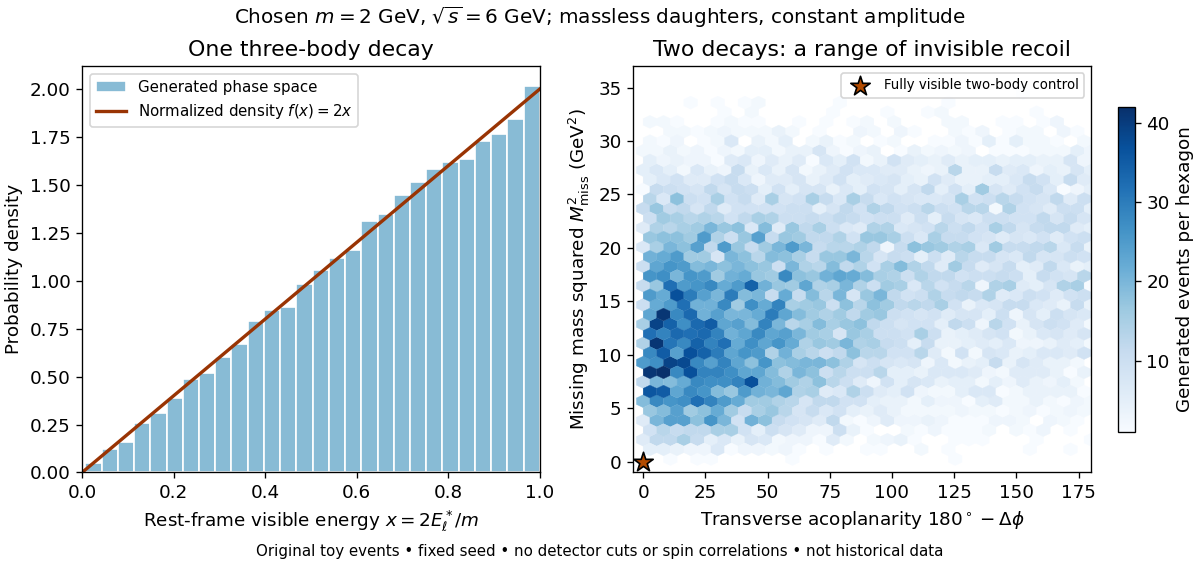
Define transverse acoplanarity by , where is the angle between the two visible momentum projections perpendicular to the beam. A fully visible two-body event with zero initial transverse momentum has and . The toy tau lepton events spread away from that point. These observables are complementary: an angular imbalance asks about directions, while the missing invariant mass also uses the visible energies and longitudinal momenta.
A Lorentz-invariant phase space density supplies allowed configurations and their geometric measure. A physical weak interaction decay amplitude reweights them and correlates spins. Consequently the plotted density is a lesson about conservation and available configurations, not a predicted experimental rate or a fit to the discovery sample. The massless charged-daughter approximation is also unsuitable near the muon rest-energy threshold.
For radial mass density within radius , integration against the spherical volume element gives . The dimensionless quantity hasThus is positive, strictly decreasing and convex, with and . Its asymptotic forms are near zero and at infinity. The density's central divergence is integrable against the factor .
In the usual physics convention for spherical coordinates, the polar angle is the angle between the positive axis and the position vector. For , it satisfies with . The north and south axes have and , respectively; the plane has . The angle is undefined at the origin. In plane polar coordinates, the same phrase usually denotes the oriented in-plane angle instead, so the reference axis and convention should always be stated. The azimuth supplies the other angular coordinate in three dimensions.
Pinned article: Introduction to the OurBigBook Project
Welcome to the OurBigBook Project! Our goal is to create the perfect publishing platform for STEM subjects, and get university-level students to write the best free STEM tutorials ever.
Everyone is welcome to create an account and play with the site: ourbigbook.com/go/register. We belive that students themselves can write amazing tutorials, but teachers are welcome too. You can write about anything you want, it doesn't have to be STEM or even educational. Silly test content is very welcome and you won't be penalized in any way. Just keep it legal!
Intro to OurBigBook
. Source. We have two killer features:
- topics: topics group articles by different users with the same title, e.g. here is the topic for the "Fundamental Theorem of Calculus" ourbigbook.com/go/topic/fundamental-theorem-of-calculusArticles of different users are sorted by upvote within each article page. This feature is a bit like:
- a Wikipedia where each user can have their own version of each article
- a Q&A website like Stack Overflow, where multiple people can give their views on a given topic, and the best ones are sorted by upvote. Except you don't need to wait for someone to ask first, and any topic goes, no matter how narrow or broad
This feature makes it possible for readers to find better explanations of any topic created by other writers. And it allows writers to create an explanation in a place that readers might actually find it.
Figure 1. Screenshot of the "Derivative" topic page. View it live at: ourbigbook.com/go/topic/derivativeVideo 2. OurBigBook Web topics demo. Source. - local editing: you can store all your personal knowledge base content locally in a plaintext markup format that can be edited locally and published either:This way you can be sure that even if OurBigBook.com were to go down one day (which we have no plans to do as it is quite cheap to host!), your content will still be perfectly readable as a static site.
- to OurBigBook.com to get awesome multi-user features like topics and likes
- as HTML files to a static website, which you can host yourself for free on many external providers like GitHub Pages, and remain in full control

Figure 2. You can publish local OurBigBook lightweight markup files to either OurBigBook.com or as a static website.
Figure 3. Visual Studio Code extension installation.
Figure 5. . You can also edit articles on the Web editor without installing anything locally. Video 3. Edit locally and publish demo. Source. This shows editing OurBigBook Markup and publishing it using the Visual Studio Code extension. 
- Infinitely deep tables of contents:




All our software is open source and hosted at: github.com/ourbigbook/ourbigbook
Further documentation can be found at: docs.ourbigbook.com
Feel free to reach our to us for any help or suggestions: docs.ourbigbook.com/#contact