Topics (374k) Articles (387k) Users (410) Discussions (242) Comments (383) Files (13k) New article
For prescribed , the steady Boussinesq top-hat plume in a stratified ambient has kinematic fluxes , , and . Balancing powers in , , and gives exponents and these positive amplitudes. The ambient's static instability is prescribed without allowing it to drive ambient motion; the Boussinesq approximation additionally requires small density differences over the modeled height range.
The intersection of a line in Plücker coordinates with a plane covector is the first displayed homogeneous vector: it lies in the span of the defining points and its contraction with is zero by antisymmetry. A zero vector means the whole line is contained in the plane. Dually, the plane through the line and a point or ideal direction is given by the second formula; it vanishes if is already on the line. These operations require no Euclidean lengths or angles.
For , a nearly circular equatorial orbit has and azimuthal frequency . The radial epicyclic frequency is , and the vertical epicyclic frequency is . Radial stability requires . The nodal precession rate is negative and the apsidal precession rate positive. These sign statements concern small eccentricity and inclination. For an arbitrary inclined orbit, the averaged argument of periapsis instead evolves as and can regress.
For a sharp thermal front moving at fraction of the Darcy velocity , a cold fluid of viscosity displacing its hot counterpart of viscosity has the displayed growth rate in the local, unbounded planar approximation without thermal conduction. The harmonic pressure perturbations decay on either side. Pressure continuity and continuity of perturbed Darcy flux give the velocity response ; the thermal front's kinematic law is . The prefactor is the thermal-front speed, not the material pore velocity. Increasing viscosity with heating therefore makes the trailing thermal interface unstable even when the leading displacement of the original fluid is stable.
The complete graph has and , exceeding the planar graph edge bound . Therefore it is not a planar graph. The complete bipartite graph has and . The general bound allows twelve edges, but the bipartite planar graph edge bound allows only eight, proving nonplanarity.
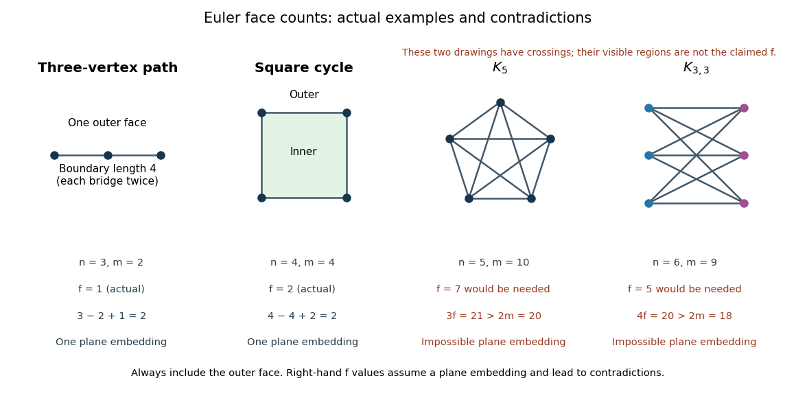
Actual plane-graph face counts compared with impossible face counts for the two complete-graph obstructions
. Details. These are necessary bounds, not a complete planarity test. For an original counterexample, subdivide every edge of once. The resulting simple graph is a connected graph with , , and is bipartite: put all original vertices in one part and all nine new vertices in the other. Both inequalities hold, and . Nevertheless, a crossing-free graph drawing would let us trace each two-edge graph path as one curve, producing an impossible embedding of . The graph subdivision preserves this obstruction. Kuratowski's theorem supplies a stronger characterization than these counts.
If a finite simple graph is a connected graph, a bipartite graph, and a planar graph, with vertices, then . Every facial boundary walk has even length and length at least three, hence at least four. Thus ; substitute the Euler formula for a connected planar graph.[ref]
Mathematics for Computer Science by Eric Lehman and others. Mathematics for Computer Science, §12.5, Lemma 12.5.2 and Theorem 12.5.3, printed pp. 486–487
The square cycle graph attains equality: . The three-vertex graph path also attains equality: . Its repeated bridges in a graph illustrate why counting facial boundary walk length correctly matters. Neither bound applies unchanged to a multigraph: two vertices may support arbitrarily many parallel edges in a plane graph.
A planar Brownian motion range has zero two-dimensional Lebesgue measure almost surely. Assuming finite expected area, Brownian scaling gives half that expected area for each half-time range. Inclusion-exclusion then makes their expected overlap zero. Translate their ranges by the midpoint position; the independent Brownian arms at a deterministic time make the expected overlap the integral of the squared point-hitting probabilities for a half-time range. Those probabilities vanish almost everywhere, so the half-time expected area, and hence the full-time expected area, vanish. This argument does not assert zero hitting probability for every individual point solely from an almost-everywhere integral conclusion.
An omitted value of a function is a point outside its image: the equation has no solution in . Both and matter. The complex exponential function on the complex plane has one omitted value in , namely zero, and two omitted values when regarded as a map into the Riemann sphere, namely zero and infinity. Restricting can create additional omitted values.
Assuming and integrating a suitably normalized polynomial times produces a positive integer that tends to zero as the polynomial degree grows. This contradiction proves that is an irrational number.
The Wallis product isIts finite product is . The Wallis integrals give , proving both convergence of the product and its value. The strict integral bounds also give .
Photon capture cross-section of a Reissner-Nordstrom black hole by  Codex 0 Created 2026-10-14 Updated 2026-10-18
For a Reissner-Nordstrom black hole with , the outer unstable circular null geodesic has radius . Maximizing for gives the critical impact parameter . The geometrical optics capture cross-section is , reducing to in Schwarzschild spacetime and in the extremal charged case. Finite-wavelength absorption need not equal this geometric limit.
// Target: general-relativity.bigb
For collisionless photons in synchronous gauge, their perturbed momentum obeys . Terms in and direction deflection times angular derivatives of are second order. Integrating the remaining linear Collisionless Boltzmann equation over gives the displayed equation, because .
// Target: cosmology.bigb
For a chain with lattice spacing and atoms, write . The periodic normal-mode condition is , equivalently for unwrapped positions. The literal position condition is incompatible with the equilibrium in that coordinate system. Fourier modes give for spring coefficient . The zero mode describes free center-of-mass translation and must be fixed or handled separately when defining an oscillator vacuum.
The Debye–Waller factor suppresses coherent scattering because atoms fluctuate about their equilibrium positions. For Gaussian displacement , the amplitude factor is and the intensity factor is its squared modulus. It multiplies the lattice interference factor, so exact extrema of the full finite-lattice intensity need not coincide with the constructive-interference centers when this envelope varies appreciably.
An information velocity must specify what counts as a newly distinguishable message and how it is detected. In a causal model, receivers cannot distinguish two otherwise identical preparations before their difference can arrive. Front velocity therefore bounds the arrival of genuinely new changes when the model has a finite domain of dependence. Group velocity can estimate the delay of a weakly distorted narrow wave packet, but it is not a universal speed of information: damping, amplification and reshaping can move the peak without advancing the first possible response. A Gaussian peak shift alone does not test relativistic causality.[ref]
Wave-Front Propagation by Richard Fitzpatrick. equations 871–873 and discussion after equation 887: earliest response versus phase propagation
The front velocity is the propagation speed of the earliest boundary of a newly introduced disturbance's support. It asks when an initially unaffected observer can first respond, whereas group velocity asks how a narrow wave envelope translates. A detector threshold defines a practical arrival time, but can miss arbitrarily small earlier responses; a packet peak is another distinct timing convention. In a causal dielectric model, a high-angular frequency contour argument gives exactly zero field for , even when phase velocity exceeds . This is a statement about that model's relativistic causality, not a universal identification of group velocity with front velocity.[ref]
Wave-Front Propagation by Richard Fitzpatrick. equations 871–873 and the paragraph following equation 887: zero field ahead of the causal front
For the stipulated Klein-Gordon equation with compactly supported real Cauchy data, front velocity is bounded by , and is the model's maximal speed of influence. A short energy method outline usesIntegration outside an expanding interval shows that zero initial energy there remains zero. Thus initial support in cannot influence before . The positive energy density includes the restoring term : this adds oscillation behind the front without extending its domain of dependence. A particular disturbance may fail to excite the leading boundary, so the maximal speed is not a promise of a detectable response for every source.
A Gaussian function is nonzero arbitrarily far away, so the Gaussian envelope in a Klein-Gordon medium has no sharp initial support boundary. Its small distant tails are already in the initial data. Likewise, keeping only a narrow interval of the frequency spectrum cannot reproduce an exact abrupt onset. Cutting off a Gaussian tail changes its Fourier transform and the accompanying initial velocity; it is a different initial-value problem. The exponential initial-velocity tail for the Klein-Gordon equation is another concrete example of a pre-existing tail outside the main disturbance.
The water-tank measurement in phase velocity records free surface elevation with calibrated resistance probes and uses a ruler and stopwatch for an independent check. The inspected protocol calls the front or back of a group a timing feature. That visible edge establishes an envelope transit estimate, not the first nonzero disturbance in the sense of front velocity.[ref]
Surface Waves Kinematics (MIT 2.016 Hydrodynamics) by Massachusetts Institute of Technology, 2.016 course staff. p. 1, Equipment; p. 2, task 2; p. 3, tasks 5–6: apparatus, calibration and group-feature timing
A proposed additional control would repeat the transit fit at several detection thresholds and train durations, using matched probe calibration and the same sampling rate. Dependence on the threshold diagnoses wave envelope reshaping or limited sensitivity; records should be compared before reflections return. Such a test could expose limitations of a group velocity estimate, but would not establish an exact causal front or validate the stipulated Klein-Gordon equation for water waves.A useful stipulated dispersive medium obeys the Klein-Gordon equation , with and . Its positive-angular frequency dispersion relation isHere is the gap at zero wavenumber, not the central angular frequency of a wave packet; the parameter in the preceding formula is . For , the phase velocity satisfies , the group velocity satisfies , and . In this stipulated medium is the limiting propagation speed of the model; it need not mean the vacuum speed of light. The same square-root dispersion relation appears in waveguide phase and group velocities, with a waveguide cutoff frequency playing the role of .[ref]
Pulse Propagation by Richard Fitzpatrick. equation 9.6 and equations 9.10–9.12: square-root dispersion and local group velocity
For the original dimensionless choice , a carrier wave has phase velocity , while a narrow wave packet has leading group velocity . After time , the carrier's zero-wave phase reference has moved to , whereas the leading wave envelope centre is at . A carrier wave crest therefore moves through the wave envelope; it does not carry an identifiable piece of the envelope with it.
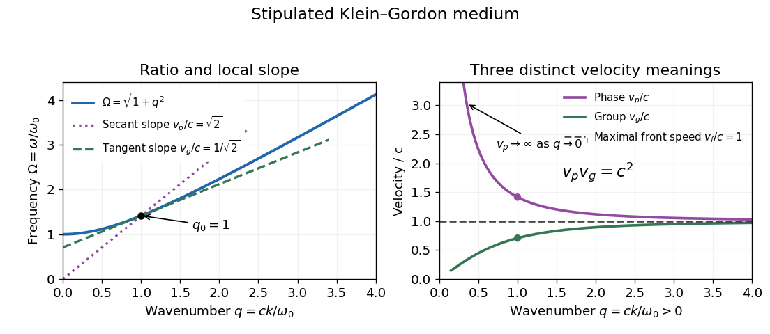
The origin-to-curve secant on the dispersion diagram gives phase velocity, while its local tangent gives group velocity. As , and ; at the phase velocity itself is undefined. As , both approach , from opposite sides. On the same positive-angular frequency branch with , both signed velocities are negative and their product remains . These conventions distinguish direction from phase speed. Reversing both and represents the same real plane wave; changing just one sign changes its direction.
For an original finite-bandwidth check, take equal-amplitude plane waves at and , still with . The exact two-tone wave envelope speed iswhile its carrier wave has phase velocity . Their product is exactly : rationalizing the difference gives . Nevertheless ; the derivative describes the limit of vanishing separation, not an arbitrary pair of tones. The two-tone wave envelope repeats indefinitely, so it has no isolated first arrival and cannot measure front velocity.
For the Gaussian functional integral with dimensionless phase stiffness and a microscopic cutoff , the Gaussian phase averaging identity gives the displayed correlation function. In two dimensions the phase-difference variance is , so the XY model has algebraic spin wave correlations with exponent . In one dimension the variance is , giving exponential decay. Above two dimensions the variance has a finite large-distance limit within the low-temperature spin wave approximation. The Laplacian Green function solves ; integration over a sphere fixes for and for . A fixed uniform phase and ultraviolet regularization are required to define itself; phase differences eliminate the constant.
Pinned article: Introduction to the OurBigBook Project
Welcome to the OurBigBook Project! Our goal is to create the perfect publishing platform for STEM subjects, and get university-level students to write the best free STEM tutorials ever.
Everyone is welcome to create an account and play with the site: ourbigbook.com/go/register. We belive that students themselves can write amazing tutorials, but teachers are welcome too. You can write about anything you want, it doesn't have to be STEM or even educational. Silly test content is very welcome and you won't be penalized in any way. Just keep it legal!
Intro to OurBigBook
. Source. We have two killer features:
- topics: topics group articles by different users with the same title, e.g. here is the topic for the "Fundamental Theorem of Calculus" ourbigbook.com/go/topic/fundamental-theorem-of-calculusArticles of different users are sorted by upvote within each article page. This feature is a bit like:
- a Wikipedia where each user can have their own version of each article
- a Q&A website like Stack Overflow, where multiple people can give their views on a given topic, and the best ones are sorted by upvote. Except you don't need to wait for someone to ask first, and any topic goes, no matter how narrow or broad
This feature makes it possible for readers to find better explanations of any topic created by other writers. And it allows writers to create an explanation in a place that readers might actually find it.
Figure 1. Screenshot of the "Derivative" topic page. View it live at: ourbigbook.com/go/topic/derivativeVideo 2. OurBigBook Web topics demo. Source. - local editing: you can store all your personal knowledge base content locally in a plaintext markup format that can be edited locally and published either:This way you can be sure that even if OurBigBook.com were to go down one day (which we have no plans to do as it is quite cheap to host!), your content will still be perfectly readable as a static site.
- to OurBigBook.com to get awesome multi-user features like topics and likes
- as HTML files to a static website, which you can host yourself for free on many external providers like GitHub Pages, and remain in full control

Figure 2. You can publish local OurBigBook lightweight markup files to either OurBigBook.com or as a static website.
Figure 3. Visual Studio Code extension installation.
Figure 5. . You can also edit articles on the Web editor without installing anything locally. Video 3. Edit locally and publish demo. Source. This shows editing OurBigBook Markup and publishing it using the Visual Studio Code extension. 
- Infinitely deep tables of contents:




All our software is open source and hosted at: github.com/ourbigbook/ourbigbook
Further documentation can be found at: docs.ourbigbook.com
Feel free to reach our to us for any help or suggestions: docs.ourbigbook.com/#contact