Topics (384k) Articles (398k) Users (410) Discussions (242) Comments (383) Files (13k) New article

For the upper half-space and the sign convention , reflect the source to and use the displayed difference. This is the negative of the conventional outgoing kernel, whose source sign is . The method of images makes the Dirichlet boundary condition zero on the plane. With and , its outward normal derivative there isThe outward unit normal is . Differentiating gives ; the real and reflected source contributions add in the normal derivative. Green's second identity therefore expresses a solution of the Helmholtz equation as when the boundary term at infinity vanishes. Suitable decay or compatible outgoing Sommerfeld radiation conditions are needed; vanishing at infinity without further control is not a general uniqueness condition for a real-frequency Helmholtz problem.
For , and the convention , the spatial Fourier transform gives the multiplier . Aligning the Fourier polar axis with gives and hence the displayed radial integral.
The pole on the integration path requires a prescription. The Cauchy principal value gives . The outgoing prescription is , yielding ; the opposite prescription gives the incoming exponential. The Sokhotski–Plemelj formula shows that the additional radial contribution is .
Let for , with real , and uniformly in direction. With sufficient boundary regularity, Green's second identity on an expanding half-ball gives the title formula. The plane integral is interpreted as the limit over expanding disks when it is not absolutely convergent. Its sign uses the upward derivative ; the outward normal derivative is .
For , and at large . The hemispherical integrand can be written , whose integral tends to zero by the Sommerfeld radiation condition. Add the boundary identities for a source point and its reflected point . On the plane and their normal derivatives are opposite. The terms involving boundary values of cancel, leaving twice and hence the title formula. In particular, zero Neumann boundary data imply in this radiating class.
For a real orthogonal involution, , so it is a symmetric matrix. Its eigenvalues are . In two dimensions the possibilities are the identity, the half-turn , and reflectionsThe reflection fixes the line making angle with the first coordinate axis and negates its perpendicular direction. This follows either from the two corresponding eigenvectors or by rotating . A nonidentity element of order two in a faithful representation must be either the half-turn or a reflection; the identity matrix is excluded by faithfulness.
Half the full range of an orbit-induced line-of-sight velocity variation, after accounting for a constant systemic offset.
One beat magnitude does not tell us the integer . In the example, every proposed optical frequency produces the same signed beat with its corresponding tooth. A coarse independent optical measurement can select the integer: once the beat sign is known, an error bound below suffices if the candidate is selected by nearest distance.
There is also a useful two-spacing check. Keep the unknown laser and fixed, track the same tooth continuously, and increase by a stipulated . Its frequency rises by , so the signed beat falls from to . HenceThis inference fails if the unknown drifts appreciably, the offset changes unnoticed, the beat sign is lost, or the tracker jumps to another tooth. The assumed tooth motion stays well below half the spacing in this example. If also changes by a measured amount, use .
For a fixed verified tooth number, the first-order frequency error is . Errors in these readings can be correlated because they share a reference. A small beat uncertainty therefore does not imply the same absolute optical accuracy: the reference's calibration and the factor remain in the error budget. A wrong tooth number is a separate discrete error, not a small correction. The beauty of the comb is that two controlled parameters organize millions of optical reference points, while the unknown's position is read electronically.
An optical fiber cutback measurement estimates distributed optical fiber attenuation by comparing a long guide with the short input portion left after cutting the output end back. Keep the launch untouched. For the following original functional model, fix wavelength, source output, input alignment and collected output cone; subtract a dark reading and keep the photodetector in its linear range. Renewed end-face quality and changed normal mode populations can still spoil the comparison. The diagram describes a measurement principle, not Kao's historical short-glass apparatus.
Let be lengths in kilometres, the corresponding positive dark-subtracted readings, and the same launch and detection factor. A uniform guide obeysHere and its estimate are numerical values in . Dividing eliminates ; taking a logarithm proves the formula. A changed instead adds an error . Reconnecting the launch between readings defeats this cancellation.
For original chosen values , , and , the predicted long reading is . The ratio gives for the removed and hence .
Suppose an unremoved additive detector background contributes to both readings. Then the apparent coefficient isThis is a bias of an estimator: a common additive background pushes the ratio toward one, whereas a common multiplicative factor cancels. For independent small zero-mean errors with standard deviations on the dark-subtracted readings, a first-order Taylor expansion givesChoosing both standard deviations as gives . A shared estimated dark offset introduces covariance, so it requires a different uncertainty calculation. Near zero signal, the logarithm and this linear approximation become unreliable.
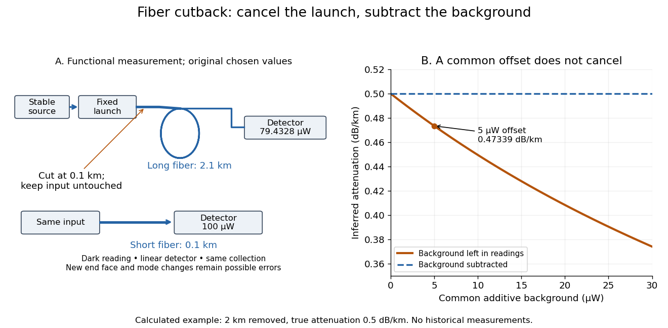
Optical fiber cutback measurement: fixed launch and additive-background bias
. Original functional schematic and calculated example. The launch stays fixed while the remote end is cut back. The graph uses the stipulated powers and lengths above; it compares dark-subtracted readings with a common positive unremoved background. No plotted point is a historical measurement. Details.An ideal operational amplifier has infinite open-loop gain and input impedance, zero output impedance, unlimited response speed and zero input offset voltage and input bias current. Its input currents vanish. In a stable linear circuit with negative feedback and a finite output, its differential input voltage tends to zero as the open-loop gain tends to infinity. Thus and are the familiar conditional circuit rules. The equality of the input voltages cannot be imposed on an open-loop, unstable or saturated circuit.
The open-loop gain of an operational amplifier is the ratio of its output voltage to its differential input voltage before an external feedback control connection is applied. A common small-signal model is , with a large direct-current gain and a dominant pole at . Above its magnitude falls approximately inversely with angular frequency.
The input offset voltage of an operational amplifier is the differential direct-current input voltage needed to make its output zero at a specified operating point. Its effect resembles a small unwanted input signal and can cause sustained output drift in an op amp integrator.
An input bias current is a direct-current component drawn by an input terminal of a real operational amplifier. Through a source resistance it produces a voltage error, and through the feedback capacitor of an op amp integrator it can produce an output ramp. Its magnitude and sign depend on the amplifier technology and operating conditions.
The slew rate bounds the large-signal output-voltage change per unit time. It is distinct from a small-signal gain-bandwidth product. A sinusoidal output of amplitude and angular frequency needs below the available slew rate to avoid this source of distortion.
An op amp integrator places a resistor between the input source and the inverting input of an operational amplifier, and a feedback capacitor between that input and the output, with the non-inverting input grounded. For an ideal operational amplifier, Kirchhoff's current law gives , henceThe initial capacitor charge supplies the integration constant. A parallel feedback resistor replaces the transfer by : the direct-current gain becomes finite while integration is recovered when . This limits offset-driven saturation. [ref]
https://wiki.analog.com/university/courses/electronics/text/chapter-2. Analog Devices, Chapter 2, integrator and parallel feedback resistance
A first-order Taylor expansion of an electrical circuit's response about an operating point. It describes small changes in electric potential difference and electric current; the neglected higher-order terms limit the useful signal range.
For , zero response before the impulse gives the displayed retarded fundamental solution. Its initial displacement is zero and its initial velocity is . The response fills the interior of the forward causal cone for the constant-speed wave equation, rather than living only on its boundary. Changing the overall sign of the differential operator changes the Green function's sign. Equivalently, the spatial Fourier transform is , whose inverse is a rectangular profile. Values assigned exactly on the wave fronts do not change the associated distribution.
The exact count is . For fixed and large , this is asymptotic to . Uniform relative accuracy requires , since the logarithm of the product starts at . The weaker assumption gives the leading sparse-link entropy but need not give a small relative multiplicity error. In the continuum range , the entropic force behaves as . The fixed-tension mean extension approaches only as the tension diverges; at the discrete endpoint the exact entropy is zero and a continuous fixed-extension derivative is not defined.
An integer pattern must survive the stated measurement uncertainty. For an original simulated example, choose a reference electric charge , define , and stipulate state meansHere each is an independent standard uncertainty of a state mean, before shared calibration effects. The generator constructs repeated noisy observations with these means; the numbers are deliberately chosen, not historical data. There is no conversion of to coulombs and no measured value of the elementary charge in this example.
For a candidate spacing in units of and proposed integers , use weighted least squares:The last two expressions follow by differentiating the quadratic in and propagating the independent errors. They are conditional on fixed, correct integer assignments and the stated error model. They do not include uncertainty from choosing those assignments. For , they give , , and . Such a small residual is compatible with this chosen error scale; it is not evidence that the errors vanish. A chi-squared distribution interpretation additionally needs the appropriate normal distribution error model and allowance for the fitted parameter; searching many assignments changes that interpretation.
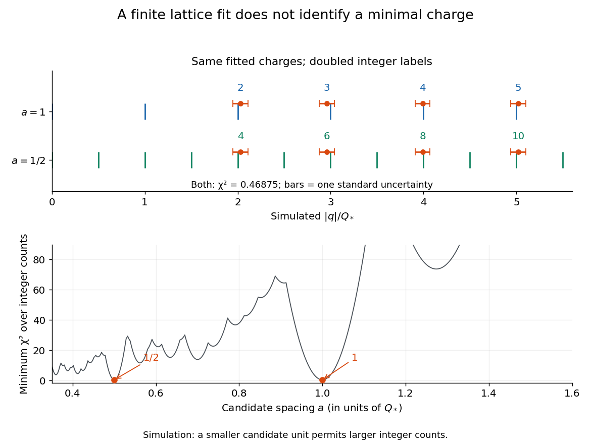
Finite noisy electric charges fit a candidate unit and its subdivisions
. Original calculation for the simulated state means above. Horizontal bars show one standard uncertainty. Both spacings and have exactly the same fitted locations and residuals when the integer labels double. The lower curve minimizes over integers separately at every candidate spacing; a low residual alone cannot identify the elementary charge. Details.The obstruction is identifiability: replacing by for any positive integer leaves every predicted reading unchanged. In particular, an -spaced pattern also fits an lattice using even indices. Even the coarsest well-fitting spacing need not be the physical unit: a dataset containing only even charge states can have twice that unit. Worse, if arbitrarily fine spacings and unrestricted integers are allowed, rounding each givesConsequently a finite fit cannot prove a minimal transferable electric charge. Reproducible smallest observed jumps supply additional evidence; interpreting them as single-carrier transfers requires independent physical support. One visibly abrupt transition could contain several unresolved transfers. In the simulation the successive differences are , , and , each with standard uncertainty . These support changes near conditional on that unit; they equally support units of . Neighboring differences share a state reading and are therefore correlated, even though the state means were stipulated independent.
A shared scale error can preserve every apparent integer relation. To first order, an independent fractional scale standard uncertainty adds to the covariance matrix of the . For the simulation, stipulating changes the conditional uncertainty of to approximately , despite the same residual pattern. Repeating timings cannot average away this common scale contribution. In the uncorrected continuum model in elementary charge, holding the other measured inputs fixed gives , so a small fractional error in air dynamic viscosity causes times that fractional error in inferred electric charge. The gas slip correction to Stokes drag requires its own propagation. Pattern agreement, drop-stability controls and absolute measurement calibration together make the inference persuasive within resolution.
Robert Andrews Millikan's 1911 protocol alternated electrically driven ascent with timed descent after short-circuiting the plates; a changed ascent speed signalled ion capture.[ref]
His 1913 refinements checked voltage before and after runs, calibrated optical distance and the clock, compared independent air-dynamic viscosity measurements, and varied pressure to test slip.[ref]
On the Elementary Electrical Charge and the Avogadro Constant by Robert Andrews Millikan. pp. 112–118
His 1924 lecture describes suppressing convection, switching the electric field, neutralizing drops, and reproducing smallest observed electrical speed increments.[ref]The Electron and the Light-Quant from the Experimental Point of View by Robert Andrews Millikan. Nobel Lectures, Physics 1922–1941; pp. 56–60
Harvey Fletcher's posthumous account recalls building the first oil apparatus and measuring with Robert Andrews Millikan; priority for suggesting oil remains uncertain.[ref]
To interpret the readout, keep one drop and one electric field polarity. Let be its signed upward terminal velocity in charge state , and let be its field-off falling speed. Use the linear drag coefficient already defined in elementary charge, with any required gas slip correction to Stokes drag included. Provided the drop's radius, surrounding air and electric field remain fixed, its electrical speed increment isThese relations apply while the electric force points upward in every state. A drop may still descend, with , when that force is too weak to support it. A held drop has and therefore , rather than zero electrical response. A neutral drop has : its signed terminal velocity agrees with field-off descent. Thus neither raw upward speed nor the ability to hold a drop is itself a count of electrons.
The ratios cancel a fixed , even if its value is poorly known. This is why relative charge quantization and absolute measurement calibration are different questions. A changed field-off warns that evaporation, air motion or another change has spoiled comparison of charge states. A stable is useful evidence but cannot exclude every compensating change. Repeat field-off checks around a proposed jump, allow the terminal velocity under linear drag to settle after switching, and propagate measurement uncertainty in both the field-on and field-off readings. Reusing a single estimate of gives the different a shared covariance.
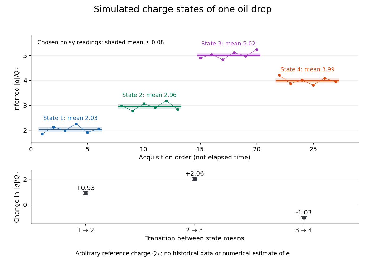
Simulated repeated electric charge states and resolved charge changes of one drop
. Original chosen noisy readings in an arbitrary reference electric charge , with four state means and their stipulated standard uncertainties. These are a simulation, not measurements by Robert Andrews Millikan or Harvey Fletcher. Acquisition order is not elapsed time; connecting lines only group observations made in the same state. Details.Consider an original ideal quantum system with positive scales andInterpret as one component of an electric dipole moment, so its coupling to the corresponding electric field is the electric-dipole interaction . The gaps are , but : this interaction has no direct first-order coupling. The nonzero squared matrix elements are and . These are coupling weights; actual spectral line intensities also depend on populations and radiation factors. In particular, there is no promise that an experiment populates the upper state of every allowed transition.
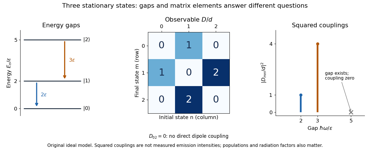
A measurement of itself has possible outcomes , sinceThese are eigenvalues of , not the energy eigenvalues . Moreover, although : two factors connect through . This algebraic statement does not turn into a nonzero direct coupling. Higher-order probability amplitudes for transitions require the appropriate dynamical calculation.
In the Heisenberg picture, an observable without explicit time dependence hasHere is the reduced Planck constant. An emitted photon on a transition with has positive angular frequency . The sign of the array's quantum phase follows its index convention; it is not a negative measured photon frequency. The frequencies involve differences of energy levels, rather than the absolute values . Adding a constant to leaves these frequencies unchanged.
Insert the complete orthonormal basis between two linear operators:The sum runs over intermediate states. The second identity follows by cancellation of ; it makes every term in the product acquire the same time factor . This is a useful reason for matrix multiplication: it composes the two indexed arrays consistently with the addition of transition frequencies. It does not multiply matching entries independently. Swapping and generally changes the intermediate-state sum and hence the result.
Pinned article: Introduction to the OurBigBook Project
Welcome to the OurBigBook Project! Our goal is to create the perfect publishing platform for STEM subjects, and get university-level students to write the best free STEM tutorials ever.
Everyone is welcome to create an account and play with the site: ourbigbook.com/go/register. We belive that students themselves can write amazing tutorials, but teachers are welcome too. You can write about anything you want, it doesn't have to be STEM or even educational. Silly test content is very welcome and you won't be penalized in any way. Just keep it legal!
Intro to OurBigBook
. Source. We have two killer features:
- topics: topics group articles by different users with the same title, e.g. here is the topic for the "Fundamental Theorem of Calculus" ourbigbook.com/go/topic/fundamental-theorem-of-calculusArticles of different users are sorted by upvote within each article page. This feature is a bit like:
- a Wikipedia where each user can have their own version of each article
- a Q&A website like Stack Overflow, where multiple people can give their views on a given topic, and the best ones are sorted by upvote. Except you don't need to wait for someone to ask first, and any topic goes, no matter how narrow or broad
This feature makes it possible for readers to find better explanations of any topic created by other writers. And it allows writers to create an explanation in a place that readers might actually find it.
Figure 1. Screenshot of the "Derivative" topic page. View it live at: ourbigbook.com/go/topic/derivativeVideo 2. OurBigBook Web topics demo. Source. - local editing: you can store all your personal knowledge base content locally in a plaintext markup format that can be edited locally and published either:This way you can be sure that even if OurBigBook.com were to go down one day (which we have no plans to do as it is quite cheap to host!), your content will still be perfectly readable as a static site.
- to OurBigBook.com to get awesome multi-user features like topics and likes
- as HTML files to a static website, which you can host yourself for free on many external providers like GitHub Pages, and remain in full control

Figure 2. You can publish local OurBigBook lightweight markup files to either OurBigBook.com or as a static website.
Figure 3. Visual Studio Code extension installation.
Figure 5. . You can also edit articles on the Web editor without installing anything locally. Video 3. Edit locally and publish demo. Source. This shows editing OurBigBook Markup and publishing it using the Visual Studio Code extension. 
- Infinitely deep tables of contents:




All our software is open source and hosted at: github.com/ourbigbook/ourbigbook
Further documentation can be found at: docs.ourbigbook.com
Feel free to reach our to us for any help or suggestions: docs.ourbigbook.com/#contact