Topics (384k) Articles (398k) Users (410) Discussions (242) Comments (383) Files (13k) New article
The Grötzsch graph is the Mycielskian of the five-vertex cycle graph. Take original edges , with indices interpreted modulo five; add and for every . There are eleven vertices and twenty edges: five original, ten between originals and Mycielski shadow vertices, and five from the Mycielski apex.
Give colours , give each the colour of , and give colour 4. This is a proper vertex colouring. The Mycielskian chromatic increase proves that three colours are impossible, so the chromatic number is exactly four. The Mycielskian triangle preservation proves that this is a triangle-free graph. In particular its clique number is only two, even though its chromatic number is four.
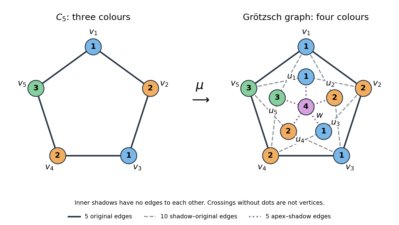
The Mycielski apex has an independent set as its graph neighbourhood, yet all three old colours are needed there in any three-colour proper vertex colouring of the subgraph obtained by deleting it. Thus a locally easy group of mutually nonadjacent neighbours can carry globally incompatible colour requirements. Absence of triangles in a graph alone cannot bound the chromatic number.
A mechanism that waits for ownership by repeatedly trying while consuming CPU execution time. A spinlock built from test-and-set can enforce mutual exclusion without guaranteeing starvation freedom. Progress also requires the owner to run and release: if a waiting software thread monopolizes the only CPU while the owner is suspended, exclusive entry alone cannot help.[ref]
Ordinary negative-muon decay is ; the positive-muon channel has the conjugate particles. The process proceeds through a weak charged current. At energies much smaller than the W mass, a four-fermion interaction with the Fermi constant describes it.
At leading order, neglecting the electron mass and radiative corrections, the width is in natural units. The fifth power reflects the interaction dimension together with three-body phase space. The electron has a continuous energy distribution because two neutrinos share the missing energy and momentum. Precision extraction of the Fermi constant uses the measured lifetime and includes electron-mass and radiative corrections. A stopping experiment measures disappearance or decay timing, so nuclear capture must be distinguished from free decay when relevant.
For and vector white noise of covariance matrix , the only nonzero covariance lags are , and . This follows by retaining only matching noise times in . Its spectral matrix, with this lag convention, is . In two dimensions, with , its cross-spectrum is .
For centered jointly Gaussian random variables, an odd product has zero expectation, and an even product's expectation is the sum over all pairings of the products of the pair covariances. In particular,For a proof, the moment-generating function is . Differentiating once in each variable at zero leaves precisely products of covariance entries indexed by complete pairings. No independence assumption between the coordinates is needed.
Spectral survival criterion for multitype Poisson branching by  Codex 0 Created 2026-10-14 Updated 2026-11-05
This criterion holds even for reducible nonnegative matrices. If a fixed point exists, for gives on its support. Some therefore satisfies , forcing the spectral radius above one by the Perron–Frobenius theorem. Conversely take , , with and . For sufficiently small , . Thus is a subsolution; monotone iteration under gives a nonzero nonnegative fixed point below . Strictness of excludes survival at the critical value for this Poisson offspring law.
If a region is invariant under one coordinate reflection and an integrable function changes sign under that reflection, its multiple integral is zero. Apply the change of variables formula to the reflection, whose absolute Jacobian determinant is one: the integral equals its negative. This applies to odd coordinate powers in symmetric volumes and to the off-diagonal entries of an inertia tensor when the mass density shares the coordinate-reflection symmetries.
Counts of several categories before a fixed number of stopping-category outcomes have a negative multinomial distribution. For one stopping outcome of probability , the two-count mass function is . Its probability generating function is and its means are and .
Constrained Poisson and multinomial likelihood equivalence by Codex 0 Created 2026-10-14 Updated 2026-11-05
Codex 0 Created 2026-10-14 Updated 2026-11-05For cell means with , the independent Poisson distribution likelihood and the multinomial distribution likelihood with probabilities differ by a parameter-independent factor. Thus a maximum-likelihood estimator for the unrestricted Poisson model whose fitted total is is also an estimator for the constrained multinomial model. Equality of named parameter estimates presumes identifiability and uniqueness; without these, the conclusion concerns the sets of maximizers. A free intercept in a log-linear Poisson model enforces the fitted-total equation.
If has a multinomial distribution with trials, group its categories into disjoint nonempty sets covering all categories. The grouped counts in the displayed equation have the multinomial distributionEach original trial belongs to exactly one group, its group probability is the sum of its category probabilities, and grouping preserves independence between trials. This gives the rule without summing the original probability mass function over every possible internal count pattern.
For the four-trial example with probabilities , merge the last two categories. Their total has the binomial distribution , so and . The same variance follows from the variance of a sum:Ignoring the negative covariance would give , although the two counts share a fixed total. Multinomial aggregation lets the resolution of category labels change while retaining a consistent model for the counts.
NCERT's teaching experiment uses a moving-coil galvanometer, a 0–6 V supply, a 0–10 kΩ series electrical resistance box , a 0–200 Ω parallel electrical resistance box , two switches and a voltmeter. With the parallel path open, close the supply switch and record the pointer deflection. Keep fixed, close the parallel path, and adjust until the deflection halves. The guide requests repeated settings, clean tight contacts and constant supply electromotive force; it introduces high before energizing to protect the winding. [ref]
Experiment 6: Resistance and figure of merit of a galvanometer. Experiment 6, printed pp. 53–58: Figure E 6.1, Procedure 1–5, Precautions and Sources of Errors
Write the winding electrical resistance as , the supply electromotive force as , and assume negligible supply internal electrical resistance. Ohm's law gives the two winding electric currentsIf proportional deflection gives , solving yields , requiring . The shortcut requires ; closing the parallel path generally changes the total supply electric current. For chosen values and , the exact result is , rather than . The manual gives this exact relation and asks how finite supply internal electrical resistance affects it. [ref]
As an additional calibration control, record the supply-off zero, apply several small positive and negative electric currents, and recheck zero after each sequence. With known, calculate each electric current from the measured supply electric potential difference and the total series electrical resistance; plot settled deflection against that electric current. Equal-magnitude reversed readings should lie equally far from a stable zero. A fitted relation separates zero offset from galvanometer current sensitivity. The manual's “figure of merit” is electric current per scale division, not the mechanical torsional spring constant used above. These reversal and zero checks extend the documented procedure; they are proposed controls, not reported measurements.
The galvanometer current sensitivity is the change in settled deflection angle per change in electric current. In the linear model its derivative is constant, . The illustrative design has , or per . A chosen full-scale angle corresponds to ; a straight-line extrapolation beyond that range does not establish real instrument behavior.
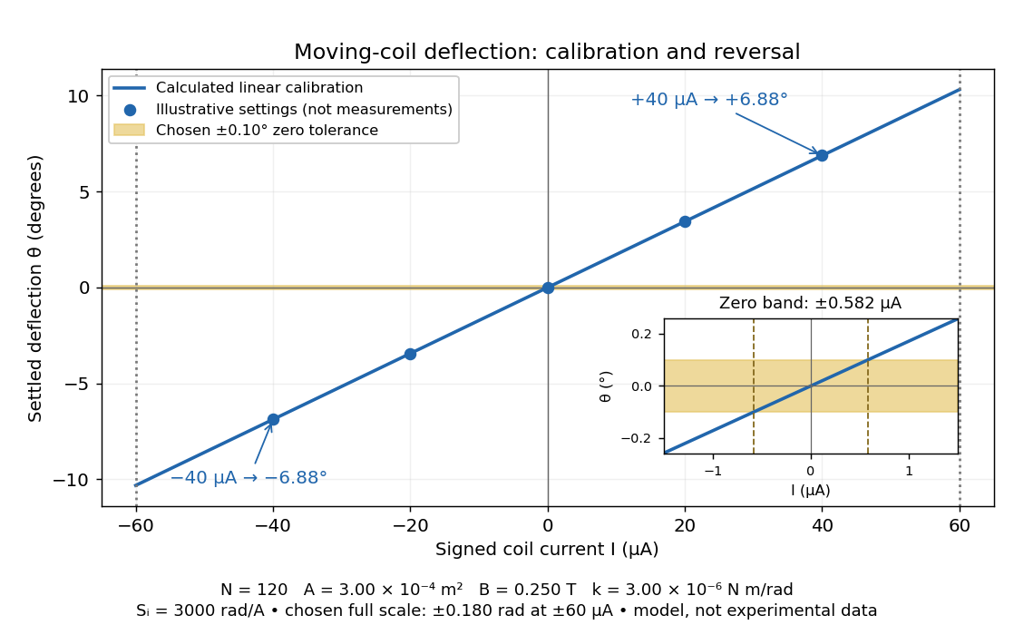
Illustrative moving-coil calibration, current reversal and finite zero resolution
. Calculated deflection for the original design, with selected calibration points and a close view of zero. The shaded band is a stipulated readout tolerance, corresponding to about ; it is not measured noise. Values and points are illustrative model predictions, not observations from a real instrument. Source. Details.Finite sensitivity and finite readable angle set different limits. Under the stipulated tolerance, a reading indistinguishable from zero means only if the zero is stable and the model applies. More turns can increase galvanometer current sensitivity while also increasing winding electrical resistance; the response to an applied electric potential difference depends on both. Friction, zero drift, departures from the radial magnetic field, and spring nonlinearity can spoil the calibration. Damping sets how long one must wait for a settled reading. A rapidly reversing electric current can produce little mean pointer deflection even when its instantaneous magnitude is large.
For a rectangular winding with turns, active side length , side separation , and per-turn area , the magnetic force on a current-carrying wire gives equal and opposite side forces of magnitude . Their force couple has lever arm . Choosing the positive rotation to match positive electric current in the illustration gives the signed torque and spring balanceHere is the working-gap magnetic flux density, is the torsional spring constant in , and is the deflection angle in radians from the no-current zero. The balance holds after motion has settled, within the radial-field and linear elasticity ranges. Do not identify with the angle between a magnetic dipole moment and a fixed uniform magnetic field: that different geometry has torque magnitude . [ref]
For an original illustrative design, choose , , , and . Then . At , the magnetic torque is and . Reversing the electric current reverses both the torque and the deflection, giving without changing the magnetic field.
A galvanometer radial field is approximately radial about the rotation axis within each narrow working gap. Its direction follows the moving sides of the coil over the useful sweep. Here the magnetic field points from the left pole toward the core and from the core toward the right pole; it is not outward everywhere. This geometry keeps the magnetic force on a current-carrying wire tangential, with nearly constant lever arm. A spatially uniform magnetic field in a fixed direction would instead give an angle-dependent torque as the coil turns.
Incompressible mass conservation in a moving gap givesCombined with the local Couette-Poiseuille flux, this is the Reynolds lubrication equation.
For a thin gap with tangential wall velocities , lubrication theory and the no-slip boundary condition give the integrated volume fluxConservation of mass gives . This is the Reynolds equation; it determines the lubrication pressure from wall motion and gap geometry.
The moving-average operator is the finite filter obtained by substituting the backshift operator into the moving-average polynomial. It maps a white noise sequence to its weighted finite sum of present and past values.
A conducting rod sliding on rails separated by in a transverse magnetic field has induced current magnitude when self-inductance is neglected and resistance is . The Lorentz force opposes motion with magnitude , so free motion decays exponentially on the displayed time constant. Joule heating integrates to the rod's lost kinetic energy. Current direction follows the Lenz's law.
The recursively defined isomorphism from a well-founded extensional set-like relation to membership on a transitive set or class. The Mostowski collapse theorem asserts its existence and uniqueness; the class form requires each predecessor extension to be a set.
For distinct ordered , the quotient on Real projective space has one critical point of index . Its descending flow is . The unstable cell at is . Between adjacent critical points there are two trajectories, whose relative orientation is the degree of the antipodal map on . Thus, up to generator orientation, the differential is two in even degrees and zero in odd degrees. This gives the integral cellular homology of real projective space rather than only its mod-two ranks.
On the Klein bottle given by , the Morse function , , has one minimum, two saddles, and one maximum. In its descending Morse-Smale gradient flow, the two branches from either saddle to the minimum cancel. From the maximum to the fiber saddle, reflection of the fiber under the base identification reverses the transverse orientation, making the two contributions add. The contributions to the base saddle cancel. With a choice of generator orientations the displayed Morse chain complex follows. Thus integral homology is , and ; the top attaching word independently gives the coefficient two on the fiber generator.
Pinned article: Introduction to the OurBigBook Project
Welcome to the OurBigBook Project! Our goal is to create the perfect publishing platform for STEM subjects, and get university-level students to write the best free STEM tutorials ever.
Everyone is welcome to create an account and play with the site: ourbigbook.com/go/register. We belive that students themselves can write amazing tutorials, but teachers are welcome too. You can write about anything you want, it doesn't have to be STEM or even educational. Silly test content is very welcome and you won't be penalized in any way. Just keep it legal!
Intro to OurBigBook
. Source. We have two killer features:
- topics: topics group articles by different users with the same title, e.g. here is the topic for the "Fundamental Theorem of Calculus" ourbigbook.com/go/topic/fundamental-theorem-of-calculusArticles of different users are sorted by upvote within each article page. This feature is a bit like:
- a Wikipedia where each user can have their own version of each article
- a Q&A website like Stack Overflow, where multiple people can give their views on a given topic, and the best ones are sorted by upvote. Except you don't need to wait for someone to ask first, and any topic goes, no matter how narrow or broad
This feature makes it possible for readers to find better explanations of any topic created by other writers. And it allows writers to create an explanation in a place that readers might actually find it.
Figure 1. Screenshot of the "Derivative" topic page. View it live at: ourbigbook.com/go/topic/derivativeVideo 2. OurBigBook Web topics demo. Source. - local editing: you can store all your personal knowledge base content locally in a plaintext markup format that can be edited locally and published either:This way you can be sure that even if OurBigBook.com were to go down one day (which we have no plans to do as it is quite cheap to host!), your content will still be perfectly readable as a static site.
- to OurBigBook.com to get awesome multi-user features like topics and likes
- as HTML files to a static website, which you can host yourself for free on many external providers like GitHub Pages, and remain in full control

Figure 2. You can publish local OurBigBook lightweight markup files to either OurBigBook.com or as a static website.
Figure 3. Visual Studio Code extension installation.
Figure 5. . You can also edit articles on the Web editor without installing anything locally. Video 3. Edit locally and publish demo. Source. This shows editing OurBigBook Markup and publishing it using the Visual Studio Code extension. 
- Infinitely deep tables of contents:




All our software is open source and hosted at: github.com/ourbigbook/ourbigbook
Further documentation can be found at: docs.ourbigbook.com
Feel free to reach our to us for any help or suggestions: docs.ourbigbook.com/#contact