Topics (384k) Articles (398k) Users (410) Discussions (242) Comments (383) Files (13k) New article
Discrete-time Markov chain martingale characterization by  Codex 0 Created 2026-10-14 Updated 2026-11-05
An adapted process on a finite or countable state space has the Markov chain transition matrix exactly when the displayed process is a martingale for every bounded test function . The forward implication follows by taking the conditional expectation of its increment. Conversely, the Martingale property gives ; testing individual-state indicators recovers the entire conditional transition law. Stopping these martingales turns equations and into hitting probabilities and expected hitting times.
A time-homogeneous Discrete-time Markov chain is a sequence of random variables indexed by nonnegative integers, with the displayed conditional probabilities. Here is its natural filtration and is a row-stochastic transition matrix. The Markov property removes dependence on earlier observations once is specified; the time-homogeneous Markov property makes independent of .
Consider states (sunny) and (rainy), with the constructed transition matrixRows give today's state and columns tomorrow's, in order . These numbers define an illustrative model, with one step interpreted as one day; they are not estimates of real weather. Let . The law of total probability gives the recurrence relationSubtracting makes the deviation multiply by at each step. ThusStarting sunny gives , , and ; starting rainy gives and . The two predictions approach the same stationary distribution while retaining a shrinking trace of the initial probability distribution.
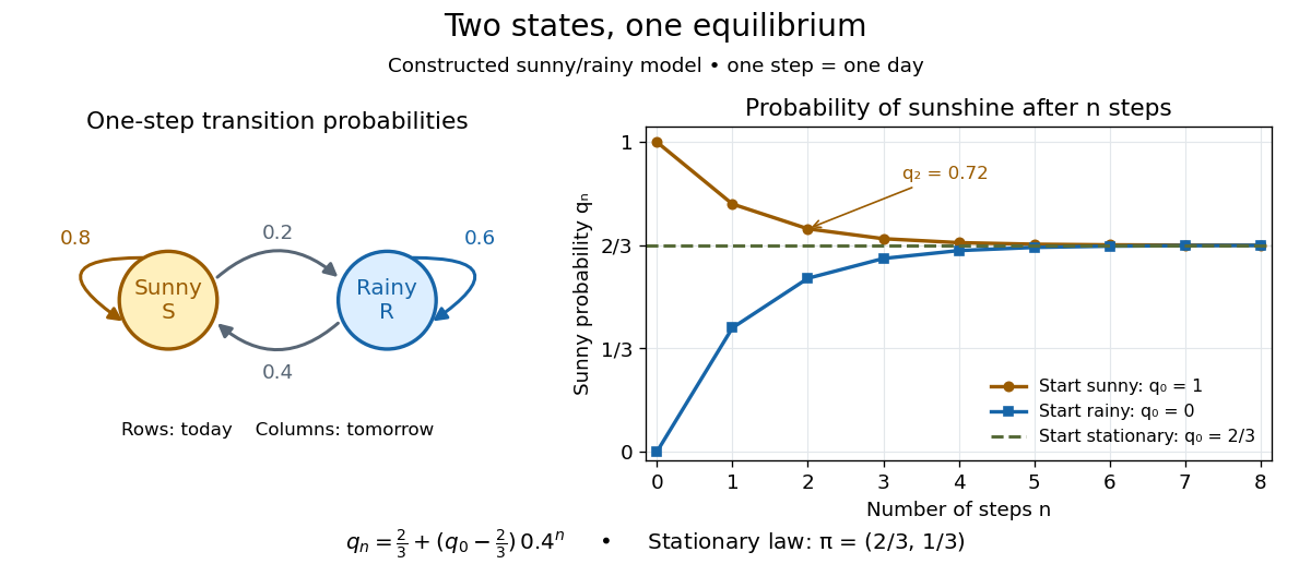
Constructed sunny/rainy transitions and the exact sunny probabilities from three initial distributions.
Details. An expected hitting time answers a different question. Starting sunny, let . Every day before the first rain remains sunny, soThis geometric distribution has finite expected value. A first-step calculation gives , with , hence days. The same result follows from the geometric series . This is a mean waiting time, not a prediction that rain first occurs exactly five days later.
A probability row vector is a stationary distribution when . The Markov chain is reversible in that law when detailed balance holds: . Multiplying those equations along a finite path gives equal forward and reversed stationary path probabilities.
Last-excursion direction law at a transient junction by Codex 0 Created 2026-10-14 Updated 2026-11-05
Codex 0 Created 2026-10-14 Updated 2026-11-05At a junction, let be the Probability that one excursion leaves through branch and never returns. If , repeated returns restart the same probabilities by the Strong Markov property. Thus the Probability of returns is , and eventual escape through is . When the branches have outward random-walk drift, the final infinite excursion tends to the corresponding end almost surely.
Fix and put . For independent geometric random variables with for , the Reflected chain with geometric downward jumps obeys . Its transition probabilities are for and .
The Probability of hitting zero from is one when and when . The first-step boundary equation at is essential for the extra exponent. Before reflection the mean increment is : downward drift corresponds to .
The chain is positive recurrent for , with Stationary distribution for . The ratio ensures these weights sum to one. It is null recurrent at and transient for . The parameter restriction matters: does not define the displayed geometric distribution, and produces deterministic upward motion rather than an irreducible chain.
For , observe a discrete-time Markov chain only when its state changes. The probability that its next different state is is . Its holding times are finite geometric waiting times. This construction deletes self-transitions and differs from the existing continuous-time jump-chain concept.
Take states for , with deterministic and transitions with probability , with probability , with probability , and with probability . The Markov chain is transient for , null recurrent for , and positive recurrent for . To see the Markov chain recurrence threshold, eliminate the primed-state hitting probabilities to obtain , with characteristic roots and . Boundedness forces return with probability one when the second root is at least one. When it is below one, the minimal nonnegative solution gives return probability from . In the positive recurrent case, put and . The stationary distribution is , and . It follows from balance across each level cut and sums to one; at criticality the invariant weights cannot be normalized.
A harmonic function assigns a value to each state of a Markov chain such that one transition leaves its expected value unchanged. This turns a question about many possible future sample paths, such as which endpoint is reached first, into a local averaging rule. For a transition matrix , a real-valued function is harmonic at state whenHere means expected value conditional on starting at ; on a countable state space the sum must be absolutely convergent. If this holds at every state, write . At an absorbing state the equation is automatic, so prescribed boundary conditions supply information that the averaging rule cannot.
For a finite Markov chain, choose a boundary set that can be reached from every state, and assign boundary values . If is its first hitting time, the harmonic extension isChoosing to be the indicator function of one target within gives a hitting probability. This is a discrete Dirichlet problem: enforce the averaging rule outside and fix the values on . See Hao Wu's MIT lecture 8, harmonic extension, slide 5. The construction extends the mean-value idea of a harmonic function; for a random walk on a graph it is a discrete harmonic function.
In mean-variance optimization with unrestricted borrowing/lending, the upper efficient ray through the risk-free point has slope . If , it touches the risky efficient frontier at the positive-premium normalized market portfolio. The Sharpe ratio there equals the slope. If this normalization is negative, the normalized tangency portfolio instead has negative excess return; the upper ray uses a short position in that portfolio and is not tangent to the upper risky branch.
Assume a positive definite covariance matrix and nonzero excess-mean vector . The Cauchy-Schwarz inequality gives , with the positive-premium efficient direction , . If , its normalized risky portfolio has Sharpe ratio . Thus negative normalization reverses the efficient orientation. If , the efficient risky direction is self-funded and cannot be normalized to a unit risky budget.
A capture-recapture model is a statistical model for repeated observations of identifiable individuals, including those missed on some occasions. A closed-population capture-recapture model estimates a fixed population cardinality; models allowing individuals to enter or leave can instead describe survival and recruitment. The sampling assumptions determine which likelihood function is appropriate.
For the two-sample closed-population capture-recapture model, condition on the sample sizes and . If the second sample selects distinct individuals from by simple random sampling, then the overlap has the hypergeometric distribution:Here is an integer and the probability mass function is zero outside these bounds. The binomial coefficients count choices of marked and unmarked individuals, divided by all equally likely size- subsets. The hypergeometric distribution has expected valueEquating the observed overlap with this expected value gives the Lincoln-Petersen estimator. The underlying sampling without replacement, probability mass function, and expected value are developed in Raymond P. Guiteras, MIT 14.30 hypergeometric distribution handout, §§1–4 and 8.
For the toy counts , , and , hold the observations fixed and vary the unknown integer . The likelihood function isValues below forty cannot contain the observed set union. Exact comparison of consecutive likelihoods gives two tied maximum-likelihood estimates, and . The Lincoln-Petersen estimator returns ; the Chapman estimator returns and is a different rule for estimation.
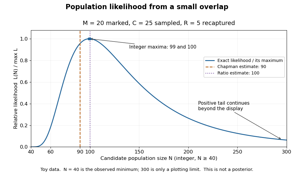
Relative likelihood for the toy overlap: integer maxima at 99 and 100, ratio estimate 100, and Chapman estimate 90
. Details. The vertical scale is . This relative likelihood compares how well candidate statistical parameters explain the same observations; it is not a posterior probability. The displayed range is only a plotting window. The likelihood function remains positive for every integer and tends to zero as increases, so the curve has a continuing right tail. The data do not justify truncating statistical inference at three hundred. The conditional hypergeometric distribution formulation also appears in Louis-Paul Rivest and Mamadou Yauck, Small Sample Estimators for Two-way Capture Recapture Experiments, §3, equation (5).
Zero recaptures require care. With and positive , the Lincoln-Petersen estimator has no finite ratio, but the capture-recapture model still gives a valid likelihood function:This likelihood function increases toward one as grows, so there is no finite maximum-likelihood estimate. For the same sample sizes twenty and twenty-five with zero overlap, forty-five distinct individuals would be observed. Lack of overlap supplies a lower bound but very weak information about large population cardinalities.
In more elaborate capture-recapture models, a first-recapture array counts individuals released at occasion and next observed at . A probability of survival and a probability of detection contribute a no-observation continuation factor . The resulting likelihood function depends on both survival and detection; these probabilities need not be separately identifiable at the last observation interval. Missing-count EM for capture-recapture describes one way to fit such a model, and identifiability remains a separate issue from computing an estimator output.
Successive mapping cones of a based map give this sequence up to homotopy. Applying based maps into a space gives an exact sequence of pointed sets in the opposite direction. The exactness statement at says that a map whose restriction to is null-homotopic extends over using the chosen null-homotopy.
Under the continuous common-distribution null of the Wilcoxon rank sum test, pooled labels are exchangeable. The product records every choice of ranks: choosing assigns rank to the first sample. Its indicated coefficient counts subsets of size and rank sum . Divide by and sum the lower tail for the one-sided P-value. Equivalently the counts satisfy with , allowing an exact integer computation.
With and no ties, sampling ranks without replacement gives the displayed mean and variance. For observed rank sum below its mean, a continuity-corrected lower-tail statistic is . Ties of sizes replace the variance by . These formulas concern the raw rank sum; the Mann–Whitney U test statistic subtracts from both the observation and its mean.
One-variable main conjecture for CM elliptic curves by Codex 0 Created 2026-10-14 Updated 2026-11-05
Codex 0 Created 2026-10-14 Updated 2026-11-05At a good split prime, the one-prime CM division tower has a pro- Galois group isomorphic to . Its prime-ramified Iwasawa module is torsion on each finite-character component. The main conjecture identifies its characteristic ideal with the corresponding elliptic-unit p-adic L-function. The class-field unit sequence and equality of characteristic ideals of global-units modulo elliptic-units and of class groups prove the identification. The cyclotomic Selmer formulation requires the appropriate CM twist and two-variable specialization; the one-prime tower is not the cyclotomic tower.
For the real p-power cyclotomic tower, take norm limits of local principal units and closed cyclotomic-unit subgroups. The corrected Coleman logarithm identifies with the Iwasawa algebra of . On a symmetric cyclotomic unit it gives . A topological generator generates the cyclotomic-unit limit and the augmentation ideal, yielding the quotient description. This local calculation does not alone identify the characteristic ideal of the global Galois module.
Characteristic-ideal bridge from local units to the main conjecture by Codex 0 Created 2026-10-14 Updated 2026-11-05
Codex 0 Created 2026-10-14 Updated 2026-11-05In the real cyclotomic tower, the class-field unit sequence gives , where is the p-ramified Iwasawa module and the unramified one. The modules are torsion over each one-variable character component. Splitting the four-term sequence into two short exact sequences proves the displayed identity by multiplicativity of characteristic ideals. The Iwasawa theorem on local cyclotomic units computes analytically. Thus the main conjecture for is equivalent to ; local interpolation alone does not prove this remaining global equality.
This lacunary series is analytic for and satisfies . At roots of unity of -power order, its radial tail diverges, giving a dense set of singularities on the unit circle and excluding algebraicity as a function. The Mahler method proves transcendence of its values at every algebraic with . At , reduced truncations have denominators and error less than twice their th power; for , the Roth theorem gives a shorter proof.
In inviscid magnetostrophic balance within an impenetrable axisymmetric container, with no azimuthal buoyancy or external mechanical torque, the cylindrically integrated Lorentz force density must vanish on every cylinder coaxial with rotation. The azimuthal pressure derivative integrates to zero, and the cylindrical Coriolis integral is proportional to net radial flux, zero by incompressibility and impermeability. Multiplying by cylinder area and lever arm gives the equivalent zero-torque form. This rotating-fluid condition is distinct from magnetic-helicity relaxation to a force-free plasma state. Its original primary source is Taylor's 1963 rotating-fluid paper.
For an imposed field in a layer of depth , the Chandrasekhar number compares magnetic tension with viscous and magnetic-diffusive effects. Here is magnetic diffusivity and is kinematic viscosity. In thermal-diffusion units the linear magnetic-force coefficient is , where and is thermal diffusivity.
Pinned article: Introduction to the OurBigBook Project
Welcome to the OurBigBook Project! Our goal is to create the perfect publishing platform for STEM subjects, and get university-level students to write the best free STEM tutorials ever.
Everyone is welcome to create an account and play with the site: ourbigbook.com/go/register. We belive that students themselves can write amazing tutorials, but teachers are welcome too. You can write about anything you want, it doesn't have to be STEM or even educational. Silly test content is very welcome and you won't be penalized in any way. Just keep it legal!
Intro to OurBigBook
. Source. We have two killer features:
- topics: topics group articles by different users with the same title, e.g. here is the topic for the "Fundamental Theorem of Calculus" ourbigbook.com/go/topic/fundamental-theorem-of-calculusArticles of different users are sorted by upvote within each article page. This feature is a bit like:
- a Wikipedia where each user can have their own version of each article
- a Q&A website like Stack Overflow, where multiple people can give their views on a given topic, and the best ones are sorted by upvote. Except you don't need to wait for someone to ask first, and any topic goes, no matter how narrow or broad
This feature makes it possible for readers to find better explanations of any topic created by other writers. And it allows writers to create an explanation in a place that readers might actually find it.
Figure 1. Screenshot of the "Derivative" topic page. View it live at: ourbigbook.com/go/topic/derivativeVideo 2. OurBigBook Web topics demo. Source. - local editing: you can store all your personal knowledge base content locally in a plaintext markup format that can be edited locally and published either:This way you can be sure that even if OurBigBook.com were to go down one day (which we have no plans to do as it is quite cheap to host!), your content will still be perfectly readable as a static site.
- to OurBigBook.com to get awesome multi-user features like topics and likes
- as HTML files to a static website, which you can host yourself for free on many external providers like GitHub Pages, and remain in full control

Figure 2. You can publish local OurBigBook lightweight markup files to either OurBigBook.com or as a static website.
Figure 3. Visual Studio Code extension installation.
Figure 5. . You can also edit articles on the Web editor without installing anything locally. Video 3. Edit locally and publish demo. Source. This shows editing OurBigBook Markup and publishing it using the Visual Studio Code extension. 
- Infinitely deep tables of contents:




All our software is open source and hosted at: github.com/ourbigbook/ourbigbook
Further documentation can be found at: docs.ourbigbook.com
Feel free to reach our to us for any help or suggestions: docs.ourbigbook.com/#contact