Topics (384k) Articles (398k) Users (410) Discussions (242) Comments (383) Files (13k) New article

Taking a finite difference lowers the degree of a polynomial phase. For , expand by shifts and apply the Cauchy-Schwarz inequality to those shift sums. This gives , where enforces that lie in . Although individual terms can be complex, the entire sum is real and nonnegative because it equals a sum of squares. For , the phase is .
For , update a local level by the displayed recursion and forecast every future horizon by . Iteration gives geometrically decreasing weights on past observations and a vanishing contribution from the initial level. It is useful for a locally stable level without a persistent trend or seasonality. A trend causes lag, motivating double exponential smoothing.
Double exponential smoothing supplements a smoothed level with a smoothed slope so that forecasts can extrapolate a local linear trend. Two common versions are Holt's linear trend method, with separate level and slope gains, and Brown's double exponential smoothing, which applies the same smoothing gain twice. They are different algorithms, not two names for one recursion. Neither version by itself models seasonal variation.
In the explicit slit map, right-side approach to gives the positive root, and left-side approach gives the negative root. The corresponding lower-half-plane boundary values are , so the two unit-circle image values are distinct. Every other conformal bijection onto the disk differs by a disk automorphism, which extends bijectively to the unit circle. Thus a sequence approaching that slit point has exactly one or both of two boundary cluster values, according to which sides occur infinitely often.
For a bounded possibly nonmeasurable real function on a probability space, its outer expectation is the infimum of expected values of measurable majorants. Its inner expectation is . They agree with the usual expected value for measurable . This permits function-space convergence in distribution for an empirical distribution process whose paths are not Borel-measurable in a nonseparable norm topology: both expectations of each bounded continuous test functional must approach its ordinary expectation under the tight measurable limiting law.
The law of the unconscious statistician computes the expected value of a measurable function of a random variable directly from the original probability distribution. If is an integrable random variable, thenUse for a probability mass function, or for a probability density function. There is no need to derive the probability distribution of first. The identity is the integration rule for a pushforward measure, and also holds with an infinite value when is nonnegative. [ref]
https://ocw.mit.edu/courses/res-6-012-introduction-to-probability-spring-2018/pages/part-i-the-fundamentals/. Tsitsiklis, Introduction to Probability, Lecture 5: the expected value rule
.For taking with probabilities , choosing gives . Its variance is therefore . Squaring the expected value would instead give , because squaring does not commute with averaging.
Hubble's law states that the instantaneous rate of change of proper distance in cosmology between comoving observers is proportional to that distance:This is exact for fixed comoving distance in an FLRW metric: differentiating gives . The dot uses cosmic time, and both distances are compared on spatial slices at the same cosmic time. The rate is not a relative velocity measured in a single inertial frame of special relativity. Thus the instantaneous relation is not an exact observed redshift-distance formula. The associated Hubble flow describes the ideal expansion; peculiar velocities describe departures from it.
For nearby sources, the observed redshift approximately satisfieswhen source and observer peculiar velocities are small compared with , additional gravitational redshift is negligible, and the changes in the scale factor and Hubble parameter during light travel are small. Here can be taken as the present proper distance in cosmology; familiar distance conventions agree at leading order in small redshift. Briefly, , while , so cosmological redshift gives . At greater redshift, use an expansion history and an explicit distance convention instead.
Stipulate the illustrative Hubble constant and speed of light . A is a million parsecs. The following are computed examples, not a catalogue of observed galaxies:
- At , and the approximate cosmological redshift is .
- At , and the approximate cosmological redshift is .
- At , and the approximate cosmological redshift is .
The displayed values are exact arithmetic under the stipulated Hubble constant; the cosmological redshift estimates use the nearby approximation and become less accurate as distance grows.
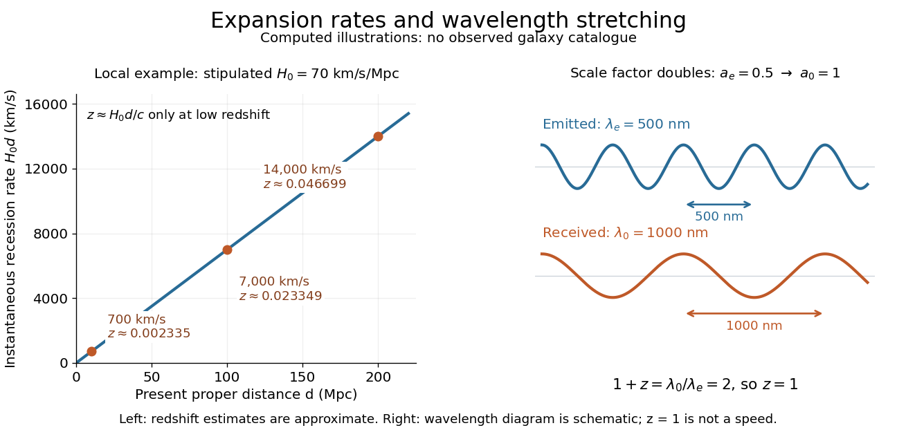
Hubble's law turns a nearby observed redshift into an approximate distance indicator and makes the uniformity of cosmic expansion tangible: twice the proper distance in cosmology means twice the instantaneous separation rate. Recentring the ideal Hubble flow on another comoving observer preserves the same proportionality, as illustrated under scale factor, so recession in every direction does not select a central observer.
In his 1929 PNAS paper, Edwin Hubble presented a relation between the distances and radial velocities of extragalactic objects. His fits gave coefficients of and for 24 individual objects and nine groups respectively, and he used about as a rounded representative value. Those historical fits used the paper's distance estimates; they are distinct from the stipulated modern-scale illustration above. [ref]
https://www.astro.puc.cl/~rparra/tools/PAPERS/hubble_1929.pdf. Hubble (1929), original PNAS paper, pp. 170-171
.For a differentiable uniformly expanding interval map, the geometric potential of an expanding map isThe exponential of its length- orbit sum is the reciprocal derivative magnitude . This weight is geometric: an inverse branch contracts interval lengths by that factor.
The corresponding Perron-Frobenius operator transports a density by summing contributions from inverse branches:For a finite smooth full-branch expanding map, standard bounded-distortion hypotheses give a positive regular fixed density , normalized by . The identity means that is an invariant measure. The cylinder averages of an invariant density explain how the geometric cylinder weights recover that density.
For the doubling map, there are two inverse branches andThe constant density is fixed, giving Lebesgue measure. Choosing an unequal-symbol potential instead produces a different Gibbs measure; an arbitrary Gibbs measure need not be absolutely continuous. Thus the potential, rather than the symbolic alphabet alone, determines whether the measure agrees with geometric length.
For the ideal Wannier-Mott exciton in energy bands whose edges occur at the same crystal momentum, the pair excitation energy, measured from the unexcited crystal, isHere is the pair's total crystal momentum; the last term is center of mass kinetic energy. For a permitted photon absorption transition with negligible recoil energy, . An electric-dipole selection rule and a nonzero transition matrix element are still needed: a bound state need not produce an observable spectral line. If the relevant energy band edges have different values of crystal momentum, a phonon can also be needed to conserve crystal momentum; subtracting a binding scale from a band gap alone does not specify the optical threshold.
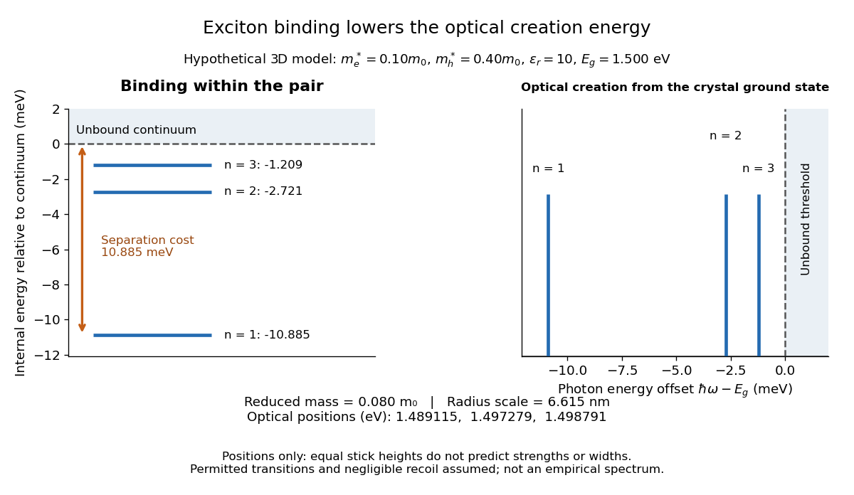
For example, the lowest internal bound state in this hypothetical model costs to create optically, yet needs only more to dissociate. The large creation energy and the small exciton binding energy answer different physical questions. An electron-hole recombination event can instead release excitation energy by photon emission or to other degrees of freedom; an emitted photon need not reproduce the original absorption energy if relaxation intervened.
A Frenkel exciton is an exciton whose internal excitation is concentrated on the scale of one molecule or unit cell. The local excitation can transfer between sites; localized internal structure does not require an immobile center of mass. The large-radius Wannier-Mott exciton approximation cannot simply be extrapolated to this limit.[ref]
Excitons in Semiconductor Quantum Dots by Matjaž Humar. §3, printed p. 6: small-radius Frenkel contrast
A Wannier-Mott exciton has an internal wave function extending over many unit cells. Its simplest model assumes a three-dimensional bulk crystal, approximately parabolic valence band and conduction band, positive isotropic scalar effective masses , a constant scalar relative permittivity , and a dilute pair population. Replace microscopic crystal forces by those effective masses and dielectric screening, and neglect exchange corrections and coupling to phonons. These assumptions must hold on the spatial and energy scales of the particular exciton.
With relative coordinate , the internal Hamiltonian operator is the three-dimensional hydrogen atom problem with a reduced mass and a screened Coulomb potential:Here is the elementary charge, the vacuum permittivity, and the reduced Planck constant. The internal energy eigenvalues, radius scale, and exciton binding energies areThe principal quantum number is . This reduction and these scales are derived in Excitons in Semiconductor Quantum Dots by Matjaž Humar (§3, printed pp. 5–6, equations (13)–(26)).
To check the scales by dimensional analysis, write , which has units of energy times length. Then is a length and is an energy. Rescaling makes , the dimensionless hydrogen atom operator. The Bohr radius is a wave function scale, not the radius of a classical orbit; for this model's lowest internal bound state, the mean separation is .
For the diagrams' hypothetical inputs , , and , where is the free electron mass, independent substitution gives , and . Here electronvolts express energy. The exciton binding energies for are approximately , and . These are model calculations, not measured material parameters. The large-radius approximation additionally requires to be much larger than the crystal's unit cell length scale. In a thin layer, with anisotropic effective masses, or with spatially varying dielectric screening, this three-dimensional formula is not generally valid.
The exciton binding energy is the positive energy needed to separate a bound electron and electron hole into the relevant unbound scattering states. Compare the exciton energy with the continuum threshold at the same total crystal momentum and for the same energy bands. The negative internal energy eigenvalue and the positive separation cost are different sign conventions for related quantities. An exciton may move freely through a perfect crystal while remaining internally bound: “free exciton” does not mean an unbound pair.
The Franck-Hertz experiment connects a reproducible loss of electron kinetic energy with excitation of a chemical atom. The original mercury-vapor experiments were performed during 1912–1914 while investigating ionization; they were not designed as a test of the Bohr model. Their later interpretation distinguished internal excitation from removal of an electron. [ref]
https://labs.physik.kit.edu/prakt-klass-physik-manuals/P2/Franck_Hertz_Versuch/. KIT physics laboratory, H23 Franck-Hertz-Versuch, Motivation
.In a modern mercury tube, a heated cathode emits electrons and a positive perforated grid accelerates them through Hg vapor. A collector slightly below the grid's electric potential rejects slow electrons. The oven controls vapor density and hence the mean free path. Keep heating and retarding settings fixed, sweep the accelerating electric potential difference , and record collector electric current . These measured quantities indirectly probe atomic excitation. [ref]
https://physlab.org/wp-content/uploads/2016/03/Franck_exp_v12015.pdf. Shah, Alam and Anwar, Electron energy loss investigated through the Franck-Hertz Experiment, sections 3–4
.The curve shows repeated current minima, typically about apart. In the collision model, an electron gains approximately of kinetic energy, with the positive elementary charge. An inelastic collision transfers about to internal excitation. Near the grid, this can prevent the electron crossing the retarding region, lowering collected electric current. Further acceleration restores collection; repeated excitation losses produce further minima. These represent multiple collisions, rather than equally spaced atomic energy eigenvalues. Contact potentials shift the first minimum, so compare several successive spacings instead of identifying the first dip's voltage with the excitation cost. [ref]
https://physlab.org/wp-content/uploads/2016/03/Franck_exp_v12015.pdf. Shah, Alam and Anwar, sections 3.1–4 and Figure 3
.The optical comparison supplies a second observable: mercury radiation at a wavelength near was detected through a window in the tube. Its inferred photon energy agrees with the characteristic collision loss, with the speed of light. This agreement supports the interpretation as a transition between internal atomic energies. It does not make the collector trace a complete spectrum. In particular, the lowest excited mercury level, labeled , is metastable because an electric-dipole selection rule forbids its direct transition to the ground state; the nearby level emits the quoted ultraviolet line. Collision excitation and optical detection therefore have different sensitivities to the available excited states. [ref]
https://ocw.mit.edu/courses/8-13-14-experimental-physics-i-ii-junior-lab-fall-2016-spring-2017/afdfff9f8bbe067239af19c8b178a764_MIT8_13-14F16-S17exp7.pdf. MIT Junior Lab, The Franck-Hertz Experiment, section VI and the discussion following Figure 6
.Initial electron kinetic energy spread and varying collision positions broaden real minima. Repeat traces at different retarding settings and oven temperatures to distinguish excitation from collection effects. This probes a discrete energy-transfer channel, rather than every energy eigenspace, its dimension, or an absolute ground-state energy. [ref].
James Franck and Gustav Ludwig Hertz presented their paper on 24 April 1914. Its heated platinum wire sat inside a cylindrical platinum mesh, with a collector 1–2 mm beyond it. A heated bath and pumping prepared the vapor; guard rings suppressed leakage. They differentiated retarding-electric current scans to study outgoing energies.[ref]
Their 1925 Nobel Prize preceded their lectures of 11 December 1926. James Franck described choosing pressure for many collisions before the mesh but few afterward.[ref]
Transformations of Kinetic Energy of Free Electrons into Excitation Energy of Atoms by Impacts by James Franck. Nobel Lectures, Physics 1922–1941; pp. 98, 100–101
Gustav Ludwig Hertz explained how a field-free collision region narrowed excitation thresholds.[ref]The Results of the Electron-Impact Tests in the Light of Bohr’s Theory of Atoms by Gustav Ludwig Hertz. Nobel Lectures, Physics 1922–1941; pp. 112, 119–120
A frequency-dependent payoff is an expected payoff depending on the population composition . Under random pairwise encounters with a fixed payoff matrix it is the linear function . The relative advantage can change sign as opponents become more or less common. The replicator equation converts this feedback into changes of frequency; nonlinear frequency-dependent payoffs allow interactions not represented by a fixed pairwise table.
The replicator equation says that a strategy grows in frequency when its expected payoff exceeds the population's current mean payoff. It is an ordinary differential equation for a composition, rather than for total population size. The subtraction of the mean is what makes relative success matter: even a type growing in absolute number can shrink as a fraction if other types grow faster.
Let be the frequency of pure strategy , with available pure strategies andIn a symmetric bimatrix game, let the payoff matrix have entry equal to the payoff to strategy against . The other player's payoff in that encounter is : symmetry between player roles does not require . Uniform random encounters give the expected payoffs and their population meanAfter choosing the time unit so that the growth-rate scale is one, the continuous-time replicator equation isHere a payoff is measured on a scale proportional to net growth per unit time, not merely as an arbitrary preference ranking. More generally one can specify locally Lipschitz frequency-dependent payoffs directly; the same equation with then defines a unique frequency trajectory. The linear pairwise model and its reproductive interpretation are given in Taylor and Jonker (1978), sections 2–3; the formulas here also follow by the following direct normalization.
Suppose the number of type obeys , where the baseline is identical for all types. Set and . The quotient rule givesThus the common baseline cancels. Adding the same constant to every entry of leaves the replicator equation unchanged; multiplying by a positive constant changes only the speed along trajectories. The same payoff matrix can therefore describe frequency evolution at different growth-rate baselines and time scales.
The probability simplex is invariant in forward time. On ,Normalization alone would not exclude negative frequencies. Nonnegativity follows as well: along a solution,An absent type remains absent, and a positive frequency remains positive at every finite time. For the fixed payoff matrix model, bounded rates on the compact probability simplex give global forward solutions. Frequencies can still tend to zero as . Each face is invariant, so this model has no spontaneous introduction of new pure strategies; mutation or outside introductions would require additional terms. For two present types the logarithm of their frequency ratio satisfies , directly expressing the accumulated payoff advantage.
For two pure strategies, write the composition as , where is the frequency of strategy 1, and letTheir payoff difference and the resulting scalar ordinary differential equation areIn the interior , the sign of the payoff difference determines the direction of motion. The endpoints are always equilibrium points, and an additional interior equilibrium point exists precisely when the affine payoff difference has a zero strictly between them. At a simple interior zero , : a negative value gives asymptotic stability, a positive value gives instability. At the endpoints and , with stability understood relative to . A zero derivative requires examining the actual flow rather than this strict sign test.
For an original coordination game, imagine two conventions that reward matching, with convention 1 giving the larger matching reward. ChooseThe crossing is . Below it, convention 1 loses frequency; above it, convention 1 gains frequency. The endpoint equilibrium points and have one-sided asymptotic stability, while is unstable: the corresponding derivatives are and , respectively. Every initial tends to , every initial tends to , and exactly stays there. Even the convention with the larger matching reward can disappear if it starts below the threshold. This is bistability, not selection of a universally best convention.
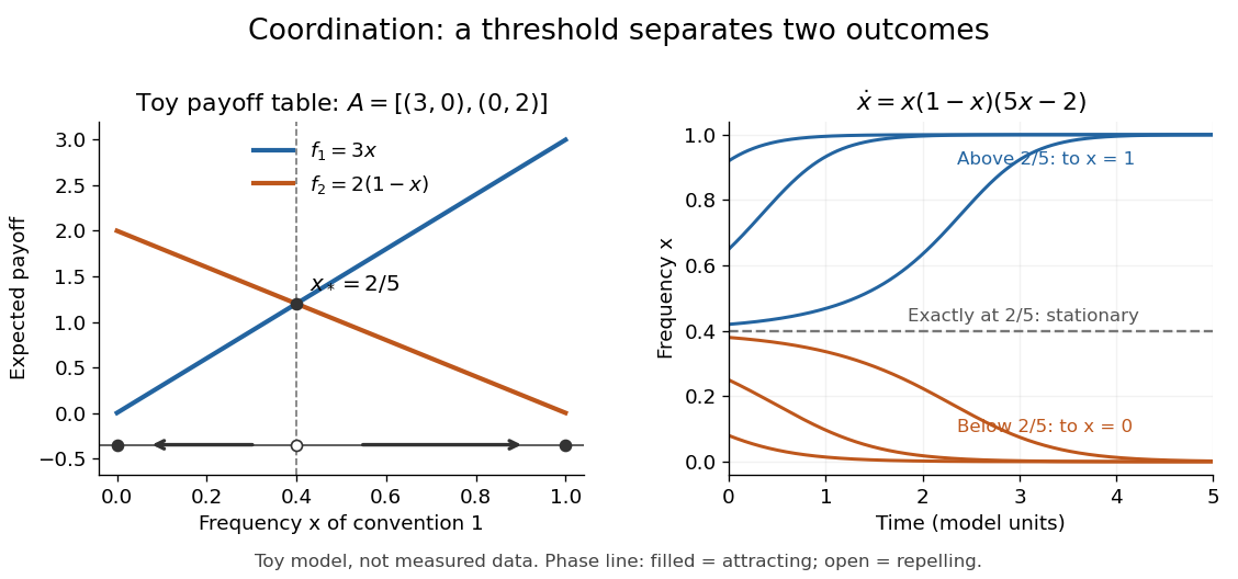
Toy coordination model: an unstable frequency threshold separates attraction to the two pure conventions
. Details. The compositions giving a symmetric Nash equilibrium in this coordination game are the two pure conventions and the mixed composition . Both pure conventions are evolutionarily stable strategies because a mutant convention has strictly lower payoff against the pure resident. The mixed symmetric Nash equilibrium is not an evolutionarily stable strategy: against that resident both conventions tie, but after a pure convention-1 mutant is introduced its payoff advantage is . Equal payoffs at a symmetric Nash equilibrium need not provide resistance to invasion or asymptotic stability.
For an original coexistence model, choose payoffs making each convention advantageous when sufficiently rare:Here attracts every initial composition with both types present: below it and above it. The interior derivative is , while and make both endpoints unstable to introduction of the other type. The endpoints nevertheless remain stationary if the other type is exactly absent; the attraction statement excludes those boundary initial states.
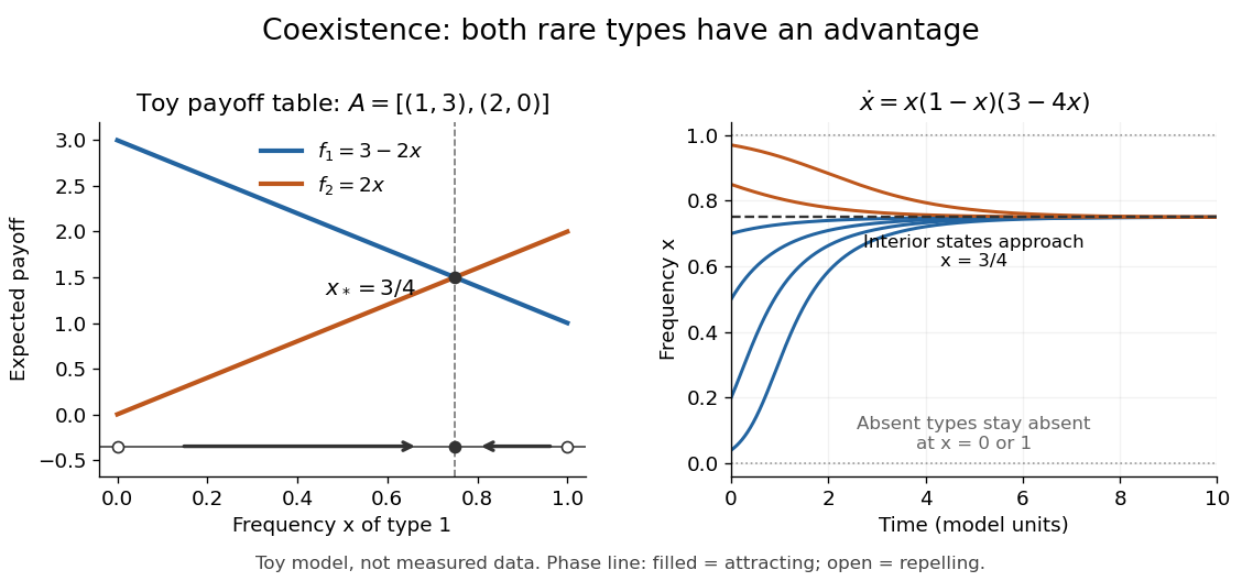
Toy coexistence model: both rare types can invade, and every interior composition approaches frequency three quarters
. Details. The sole symmetric Nash equilibrium in this coexistence model is . It is also an evolutionarily stable strategy. For any different mixed strategy , the first comparison in the two-condition criterion for evolutionary stability ties because . Its second comparison is strictly positive:Thus restoring frequency feedback can protect a mixture even though all present types earn equal payoffs at the mixture. Coexistence here means different individuals using different pure strategies; it does not require every individual to randomize with a mixed strategy.
Frequency evolution need not increase the mean payoff. In the coexistence example , whose maximum occurs at , whereas the attracting composition is . For , the frequency increases while . Individual payoff advantages drive the equation; maximizing collective mean payoff is a different optimization problem.
More generally, a rest point only equalizes payoffs among present types: implies . A symmetric Nash equilibrium additionally requires for every absent type. All vertices are rest points even when an absent type could invade. For finite symmetric bimatrix games, a rest point with Lyapunov stability on the full probability simplex is a symmetric Nash equilibrium; an interior trajectory that converges has a symmetric Nash equilibrium as its limit. These are conditional results, not a convergence theorem for every trajectory. See Cressman and Tao (2014), Theorem 1.
The rock paper scissors payoff matrix gives an explicit obstruction to universal convergence:Since , , and in the interior . Thus is conserved. Its maximum on the probability simplex occurs only at , the unique symmetric Nash equilibrium, so an interior trajectory starting elsewhere cannot converge to that composition. Every other interior product level is a closed curve without a rest point, giving a periodic orbit. The existence of these cycles is also discussed in Cressman and Tao (2014), Example 1. The useful lesson is to inspect the specified payoff feedback and dynamical system, rather than infer convergence from the existence of an evolutionarily stable strategy or a Nash equilibrium.
For mixed-strategy expected payoffs put and . The invasion payoff difference is exactly . Positivity for all sufficiently small positive forces by taking the limit. When , it forces . Conversely makes the difference positive for sufficiently small frequency, and makes it positive for every positive frequency. Apply this separately to every distinct mutant. This proves the equivalence with an evolutionarily stable strategy; affineness in population composition is essential to the formula.
Hawk fights for a resource of value , while Dove retreats from Hawk and shares with another Dove. Hawk–Hawk competition incurs damage cost . The expected payoff difference between Hawk probabilities against population probability is . For positive , pure Hawk is an evolutionarily stable strategy when . At , it remains stable because a mutant loses against its own population. When , the stable mixture has Hawk probability : all first-condition payoffs tie, and its second-condition advantage is . For nonpositive resource values, pure Dove is stable if or if . At all payoffs vanish and there is no evolutionarily stable strategy.
For a differentiable rare-mutant invasion fitness against resident trait , the selection gradient gives the first-order growth advantage of a nearby mutant. A zero gradient is a candidate interior evolutionary singularity. Strict local uninvadability follows from negative mutant-fitness curvature; evolutionary approach additionally requires the gradient to point toward the candidate. Boundary traits require one-sided tests. A gradient alone does not prove global evolutionary stability.
Every event in complete Minkowski spacetime emits a future-directed null geodesic ending on future null infinity. Therefore its black-hole region is empty and there is no intrinsic event horizon. The null edges of the Minkowski conformal compactification represent infinity, not hidden regions inside the physical spacetime. An accelerated observer can instead have an observer-dependent Rindler horizon.
An Eulerian trail, also called an Eulerian path, is a trail in a graph traversing every edge exactly once. The name Eulerian path does not require a graph path: vertices may repeat. A Hamiltonian path instead visits every vertex exactly once, and may omit edges. An Eulerian trail may omit isolated vertices, so these are different coverage requirements.
For a finite undirected multigraph with at least one edge, allowing self-loops, an Eulerian trail exists exactly when the edge support of a graph is a connected graph and there are zero or two vertices of odd vertex degree. In the two-odd-vertex case they must be the two distinct endpoints; in the zero-odd-vertex case every Eulerian trail is an Euler circuit. Count a self-loop twice in the vertex degree but once in the trail, and count each parallel edge separately.[ref]
Math 530 Spring 2023, Lecture 6: Multigraphs and digraphs. pp. 1–3, Theorem 1.1.2 and the note about isolated vertices
The parity obstruction is local: each intermediate visit pairs an arriving edge with a departing edge. Only the distinct endpoints can have an unpaired incidence. The handshaking lemma, , also shows that the number of vertices with odd vertex degree is even. Sufficiency in the two-endpoint case reduces to the Euler circuit criterion: add one extra edge between the odd vertices, construct an Euler circuit, rotate its record to start with the extra edge, then delete that edge. The remaining trail has the required endpoints.
For the Seven Bridges of Königsberg multigraph, the vertex degrees at are , so no Eulerian trail exists. Remove the unique edge : the vertex degrees become , and a six-edge Eulerian trail runs from to . Label the parallel edges between and between ; label by and by . A complete record is . It revisits while using every remaining edge once.
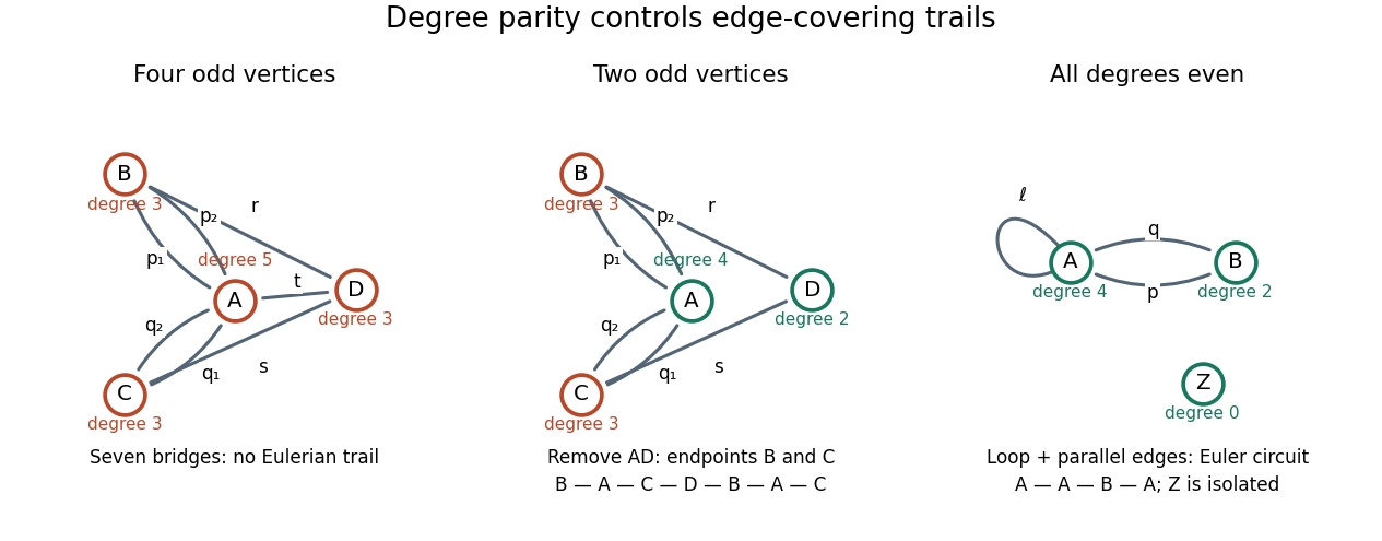
Four odd vertex degrees forbid an Eulerian trail; two allow distinct endpoints; zero allow an Euler circuit
. Details. Pinned article: Introduction to the OurBigBook Project
Welcome to the OurBigBook Project! Our goal is to create the perfect publishing platform for STEM subjects, and get university-level students to write the best free STEM tutorials ever.
Everyone is welcome to create an account and play with the site: ourbigbook.com/go/register. We belive that students themselves can write amazing tutorials, but teachers are welcome too. You can write about anything you want, it doesn't have to be STEM or even educational. Silly test content is very welcome and you won't be penalized in any way. Just keep it legal!
Intro to OurBigBook
. Source. We have two killer features:
- topics: topics group articles by different users with the same title, e.g. here is the topic for the "Fundamental Theorem of Calculus" ourbigbook.com/go/topic/fundamental-theorem-of-calculusArticles of different users are sorted by upvote within each article page. This feature is a bit like:
- a Wikipedia where each user can have their own version of each article
- a Q&A website like Stack Overflow, where multiple people can give their views on a given topic, and the best ones are sorted by upvote. Except you don't need to wait for someone to ask first, and any topic goes, no matter how narrow or broad
This feature makes it possible for readers to find better explanations of any topic created by other writers. And it allows writers to create an explanation in a place that readers might actually find it.
Figure 1. Screenshot of the "Derivative" topic page. View it live at: ourbigbook.com/go/topic/derivativeVideo 2. OurBigBook Web topics demo. Source. - local editing: you can store all your personal knowledge base content locally in a plaintext markup format that can be edited locally and published either:This way you can be sure that even if OurBigBook.com were to go down one day (which we have no plans to do as it is quite cheap to host!), your content will still be perfectly readable as a static site.
- to OurBigBook.com to get awesome multi-user features like topics and likes
- as HTML files to a static website, which you can host yourself for free on many external providers like GitHub Pages, and remain in full control

Figure 2. You can publish local OurBigBook lightweight markup files to either OurBigBook.com or as a static website.
Figure 3. Visual Studio Code extension installation.
Figure 5. . You can also edit articles on the Web editor without installing anything locally. Video 3. Edit locally and publish demo. Source. This shows editing OurBigBook Markup and publishing it using the Visual Studio Code extension. 
- Infinitely deep tables of contents:




All our software is open source and hosted at: github.com/ourbigbook/ourbigbook
Further documentation can be found at: docs.ourbigbook.com
Feel free to reach our to us for any help or suggestions: docs.ourbigbook.com/#contact