
Past exam of the quantum condensed matter course of the University of Cambridge 2017 4 Solution 2026-10-18
Noninteracting spectral line. Treat as a wavevector, so physical crystal momentum is . Write ; an energy zero at the chemical potential can be chosen throughout. The temporal factor of a noninteracting state is . With the Fourier transform convention ,Thus its normalized frequency spectral function isOne should not square the delta distribution as if it were an ordinary finite-time transition amplitude. More precisely, the fermionic retarded Green function is . Its Fourier transform is , whose negative imaginary part divided by is the same delta peak.
Interactions and lifetime. Interactions change the dispersion through the real part of the self-energy and permit decay into other excitations through its imaginary part. In the simplest quasiparticle-pole model, exponential decay of the retarded amplitude givesPerforming the causal integral,The corresponding Lorentzian quasiparticle spectral peak isIts total frequency integral is one. The exponential amplitude lifetime is ; the probability lifetime is . Describing as a scattering rate therefore requires the lifetime convention to be specified. The energy half-width is .
A general interacting Electron is more accurately described by near the pole. The coherent peak then integrates to the quasiparticle residue and an incoherent continuum carries the remaining weight. In an energy-unit self-energy convention,Linearizing the real denominator gives and at the pole. The requested unit-weight Lorentzian is the normalized quasiparticle model, not the most general exact interacting spectrum.
Peak position and width. At fixed , put and . Differentiation givesIt is positive for and negative for , so the only maximum is at , with height . Setting to half this height gives . ThereforeIn energy units the maximum is and the half-width is . Frequency dependence of the self-energy would require reconsidering both the shape and peak position.
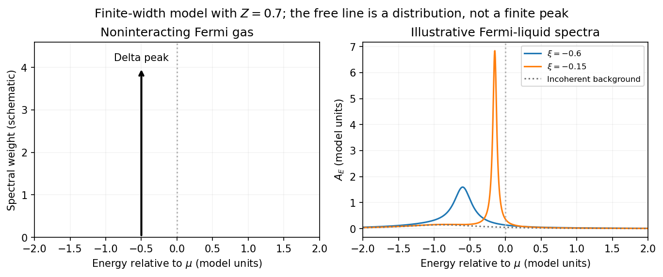
Fermi gas and Fermi liquid. A noninteracting Fermi gas has a delta-function spectral line at its bare dispersion for every momentum. A normal three-dimensional Fermi liquid has a shifted coherent peak plus incoherent spectral weight; close to the Fermi surface its width scales as . At zero temperature the peak becomes arbitrarily sharp at the Fermi surface, while it broadens farther away. Spectral functions include addition and removal weight; occupied-only photoemission contains an extra Fermi factor.
Photoemission measurement. A photon of known energy ejects an Electron. Measure its kinetic energy and emission direction. For binding energy below the Fermi level and the appropriate calibrated work function , conservation of energy givesConservation of momentum parallel to a periodic surface giveswhere is a surface reciprocal-lattice vector. At suitable photon energies the photon momentum can be neglected; at higher energies it must be retained. The surface breaks perpendicular translation symmetry, so the perpendicular crystal momentum generally needs a final-state model. A two-dimensional band can be reconstructed directly from the parallel components.
Within the sudden approximation and electric-dipole approximation, photoemission intensity and spectral function are related byHere is measured relative to the chemical potential. Instrumental resolution convolves the product and inelastic scattering adds background. Thus ARPES maps the occupied electron removal spectral function, weighted by a matrix element; it does not measure the full unoccupied spectrum or an unweighted spectral function automatically. Bright ridges give dispersions, and intrinsic widths give decay information after instrumental effects are removed.
Reading the supplied image. Its bright ridges form a graphene-like cone. The crossing near is the Dirac point, not in general the Fermi level. In the paper's plotted energy coordinates its energy is roughly –. A velocity follows from a branch slope independently of the energy zero:For example, the lower branch moves by about between and . This gives andReading other points changes the estimate by tens of percent. The original exam image has unequal energy increments on nearly equally spaced labelled ticks, so it does not justify a precise fitted velocity. The value is an estimate of the cone slope extrapolated to the Fermi crossing, rather than a measured derivative exactly at a visibly identified Fermi cutoff.
To determine a Fermi energy, first calibrate the Fermi edge, then subtract the chosen reference energy. Neither a Fermi-level marker nor an explicit energy-zero convention is supplied in this crop. If its upper termination near is intended to represent the Fermi cutoff, the conditional graph answer is on that axis, or relative to the Dirac crossing. Identifying the crossing itself as the Fermi energy would incorrectly assume undoped graphene.
The research article cited by the exam identifies this as linearly polarized graphene ARPES and independently states for the substrate-doped sample. That resolves the relative energy when this external calibration is admitted.[ref]
https://hrg.pusan.ac.kr/articles/JPCM_0953-8984_26_33_335501.pdf. Section 3, printed p.2 and figure 1(b): Dirac point below the Fermi energy
The crop alone does not uniquely fix an absolute Fermi energy; the source-supported relative value and the conditional axis reading should be distinguished. Past exam of the quantum condensed matter course of the University of Cambridge 2017 3 Solution 2026-10-18
Band edges and optical transitions. A direct band gap has the conduction minimum and valence maximum at the same crystal momentum. A near-edge photon then connects the two almost vertically on an energy-versus-wavevector plot, because its momentum is small on the Brillouin zone scale. An indirect band gap has the extrema at different momenta, so an additional momentum transfer, commonly supplied by phonon absorption or emission, is required for a near-edge radiative transition. This reduces its probability relative to an allowed direct transition.
Near the zone centre, an isotropic direct-gap model has and downward valence dispersions . The heavy-hole and light-hole bands are the upper branches with large and small positive hole masses: the heavy branch is flatter. In common cubic semiconductors these arise from the manifold, while spin-orbit coupling places the split-off valence band lower by . Its thermally generated hole population is suppressed by approximately relative to upper-valence holes, apart from density-of-states factors. Neglect is justified when ; it is not a universal exclusion of this band at arbitrary temperature.
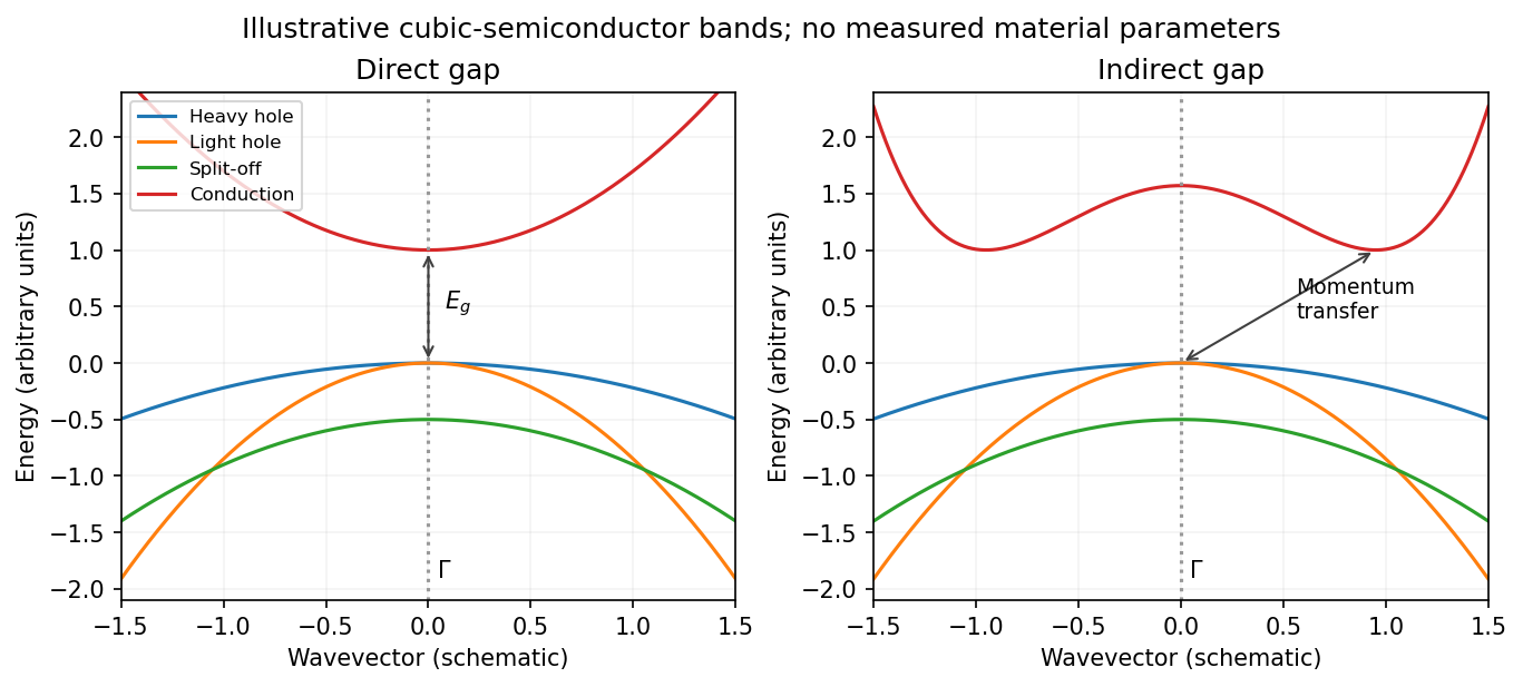
Original schematic direct and indirect band edges, including heavy, light and split-off hole branches
. Details. For an indirect material such as Si, the conduction minimum need not be at . In applying the carrier-density formulae, must mean the actual minimum of the included conduction valley. The supplied scalar effective masses and densities of states constitute a simplified band-edge model; they do not specify Si's full valley anisotropy or multiplicity.
Carrier populations. Let be the Fermi-Dirac distribution. In the nondegenerate conduction tail, . Set and integrate the given density of states:The integral is . Defining the effective density of states givesThe factor two is already included in the supplied density of states; it must not be added a second time.
A hole is an unoccupied valence state. For sufficiently below , . Substitution of gives in exactly the same wayTheir product eliminates the chemical potential:This is the semiconductor mass-action law at thermal equilibrium. In an intrinsic semiconductor, charge neutrality additionally givesIn a doped semiconductor the product still applies in this nondegenerate equilibrium model, but the two populations need not be equal.
Intrinsic chemical potential. Taking logarithms of yields the intrinsic-semiconductor chemical potentialFor unequal band degeneracies, use the first form with the full . For the supplied mass ratio , the shift from midgap at is approximately , toward the valence edge.
Three temperature regimes. The original plot runs from high temperature on the left to low temperature on the right. At high temperature, thermal excitation across the gap dominates and rises rapidly with temperature. In the middle, donors and acceptors are effectively ionized, the material is extrinsic, and makes the plateau. At low temperature, dopant freeze-out binds increasing numbers of Electrons to donor levels, reducing the mobile-electron population as the sample cools. Its activation scale is a donor binding energy, not the full band gap. Compensation and incomplete ionization affect that regime.
Gap estimate from the original figure. On the dashed intrinsic branch, . Hence band-gap extraction from intrinsic carrier activation uses the slope of versus . With and expressed in eV/K, two points giveThe very compressed intrinsic branch is only approximately readable: near and near . These give , rather than a precision determination. Neglecting the thermal prefactor gives about from those same rough points. Thus a gap of order – is justified by this schematic plot; its resolution does not support distinguishing a few hundredths of an electronvolt. The declining freeze-out branch must not be used to infer the full gap.
Room-temperature densities. At , the supplied masses giveIn the fully ionized extrinsic plateau, put . Charge neutrality and the mass-action law implySince , is insensitive to the imprecise gap. The minority density is much more sensitive:Using gives and . Using instead gives and . These are explicitly conditional estimates within the stated mass model. The plot alone cannot fix a precise minority density because the uncertain gap occurs inside an exponential.
Past exam of the quantum condensed matter course of the University of Cambridge 2016 4 Solution 2026-10-18
Relaxation-time model. The Drude model treats mobile charge carriers as independent particles accelerated by the Lorentz force between scattering events. Collisions randomize the drift momentum toward local equilibrium and are represented by a uniform, field-independent momentum relaxation time. For the present calculation the carrier density, isotropic mass and relaxation time are fixed, the fields are uniform and stationary, and quantum orbital quantization and intercarrier correlations are neglected. The steady drift velocity obeysHere is the number of carriers of that species per unit volume, their signed charge, their inertial or isotropic band mass, the momentum relaxation time, and their single-species electrical conductivity at zero field.
One-carrier tensor. With and , solving for the electric field givesSince and ,Thus the resistivity tensor, defined by , isIts off-diagonal signs follow from the stated axes and signed . For zero transverse electric current, is the Hall electrical resistivity; reversing charge reverses it. The single-species longitudinal electrical resistivity is independent of in this ideal isotropic model.
Adding Electrons and electron holes. Let both species have density and charges , with . The stipulated equal zero-field electrical conductivity means equal positive charge carrier mobility , even if their masses and momentum relaxation times separately differ. Put and . Inverting each electrical resistivity matrix givesBoth species experience the same electric field, so their electric current densities add. Therefore it is their conductivity tensors, rather than their resistivity tensors, that must be summed. The Hall parts cancel andThis is compensated two-carrier magnetoresistance. Although the net Hall field vanishes, each carrier species is bent in its own direction; maintaining the total longitudinal electric current requires an increasing longitudinal field. Equal carrier numbers alone do not ensure zero Hall response if charge carrier mobilities differ; both equalities given here are used.
Large-field limit and quantum oscillations. Expanding the exact diagonal entry,For ,Here the last equality applies to either species with its own mass and transport time; the stipulated charge carrier mobilities give the same threshold. This is the classical strong-field condition : carriers turn substantially before their drift momentum relaxes.
Observable quantum oscillations additionally require sufficiently sharp Landau levels and a sufficiently cold Fermi-Dirac distribution, approximatelyWhen , the disorder field scale is comparable to the onset scale for large classical magnetoresistance. The thermal condition can demand a much larger field, and when even the disorder criterion is stronger. The quantitative damping factors in Q2(c) show that these are crossover scales rather than sharp visibility boundaries. A large smooth magnetoresistance therefore does not itself demonstrate Landau level; it can exist while thermal smearing suppresses oscillations. Conversely, the asymptotic condition is stronger than merely reaching unity, so there is no universal ordering of the two experimental onset fields without temperatures and lifetime information.
Scaling function. The material's actual zero-field longitudinal electrical resistivity is . Dividing the exact answer by this value givesThe assumption that stays constant is essential to eliminating further temperature-dependent parameters. is a dimensionful scaling variable; is its dimensionless version. The corresponding fractional increase is .
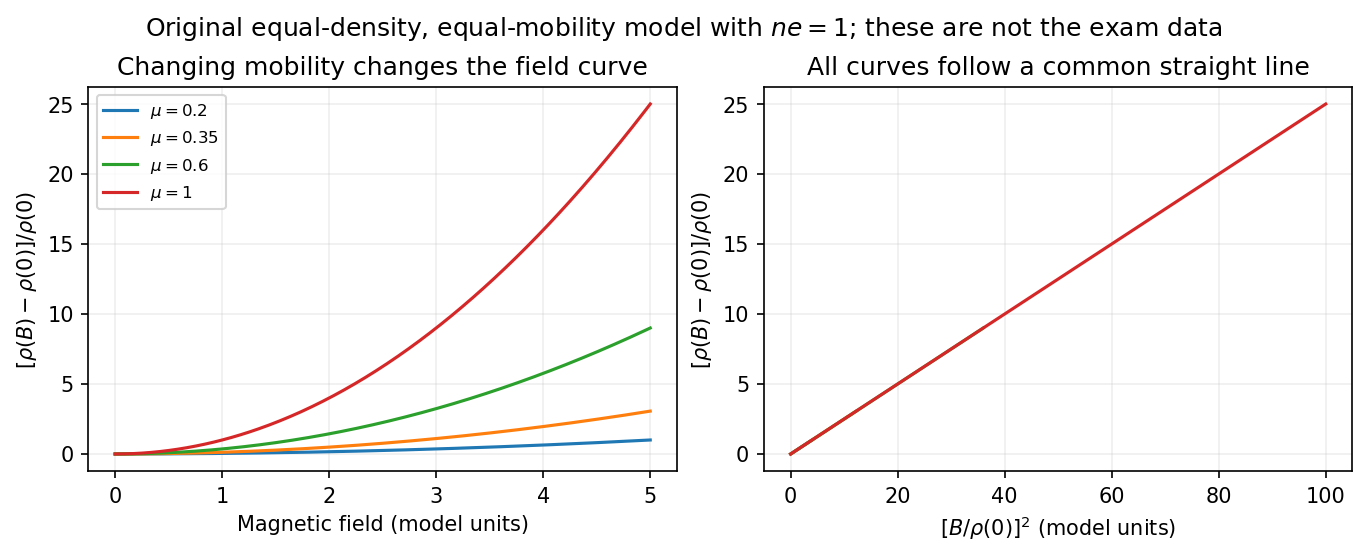


What the supplied data test. In the original PDF's left panel, the field dependence is strongly temperature dependent. In the right panel, plotting the fractional magnetoresistance against the squared rescaled field makes the displayed 125, 150, 175, 200 and 225 K curves collapse approximately onto one straight line, over the field intervals where they overlap. This supports the proposed one-parameter scaling and, on that range, the quadratic field law. The 100 K curve does not collapse: it bends away and has a different slope in the rescaled plot. The indicated scaling is therefore supported for the displayed 125–225 K data, not for the entire displayed temperature range. The graph alone does not locate a sharp transition between 100 and 125 K or establish behavior above 225 K.
This empirical collapse is Kohler's rule. It is consistent with a common temperature-dependent charge carrier mobility or relaxation scale and a fixed carrier population; it is not a unique proof of exact compensation or of one microscopic scattering mechanism. A change in relative scattering times, carrier population or Fermi-surface structure could spoil the collapse, and this figure alone does not select the cause of the 100 K departure.
There is a factor-of-two normalization convention in the printed text. The introduced for each species gives , whereas the final paragraph calls “.” If denotes the experimentally measured zero-field electrical resistivity, the consistent slope isIf one instead keeps the literal single-species definition , the same model has . The choice rescales and offsets the axes by temperature-independent constants, so it does not change which temperature curves collapse, but it must be resolved before inferring a carrier density from the slope.
Past exam of the quantum condensed matter course of the University of Cambridge 2016 3 Solution 2026-10-18
mass as band curvature. In a periodic potential, a weakly forced Electron is usefully described by a wave packet confined to one energy band. Its group velocity isDifferentiating the velocity givesThis effective-mass tensor describes the band response, not a change of the Electron's bare rest mass. Along a principal direction, a steep upward curvature gives a small positive mass and a flatter curvature a larger one. Near a band maximum the Electron curvature and effective mass are negative; the corresponding missing-electron description uses positive electron hole masses. Anisotropy produces distinct principal masses, and strong nonparabolicity makes them momentum dependent. The single-band semiclassical description assumes fields weak and slowly varying enough to avoid substantial interband transitions.
Lattice symmetry and Bloch's theorem. Use the active spatial translation operator . A lattice-periodic scalar potential satisfies , while the kinetic term is translation invariant. Therefore . The lattice translations also commute with one another, so they can be diagonalized simultaneously with , including within a degenerate energy subspace.
For a common eigenstate, write . Unitarity gives , and the group law gives . On primitive Bravais vectors , choose . Every lattice vector is an integer combination of these generators, henceThe vector is defined modulo a reciprocal lattice vector. The band index labels the different energy eigenstates with the same translation character. Define . The phase factors cancel under a lattice translation, proving Bloch's theorem in its usual form:This is the Translation-character proof of Bloch theorem; the commutator guarantees a basis of such states, even when an arbitrary superposition of different translation characters is not itself a translation eigenstate.
Periodic Hamiltonian. Acting once with momentum gives . Applying it again and cancelling the common plane-wave factor yieldsThe Bloch Hamiltonian acts on lattice-periodic functions in a unit cell. Expanding its square separates a zero-momentum Hamiltonian, a term linear in and an identity term quadratic in .
Expansion about the zone centre. Let , , and normalize all these states using a unit-cell inner product. For the real scalar Hamiltonian in the question, a nondegenerate zone-centre eigenfunction can be chosen real. Thenbecause opposite unit-cell faces cancel. Equivalently, time-reversal symmetry forbids a nonzero electric current in this nondegenerate spinless state. This explains why no linear energy term appears; it should not simply be omitted without a symmetry or extremum argument.
The first-order energy shift is therefore . In the second-order sum the quadratic term is proportional to the identity and has no off-diagonal matrix elements. Only the linear momentum vertex contributes. Second-order nondegenerate perturbation theory gives the momentum matrix-element expansion of band energyHermitian operator makes the two reciprocal matrix elements complex conjugates. All other periodic eigenstates at enter the sum. The remainder is even because time-reversal symmetry gives near this isolated state. At a degeneracy the denominators signal the need for degenerate perturbation theory instead.
mass ratio and the printed formula. Write . Differentiating the quadratic energy yieldsFor a specified unit direction , the resulting scalar mass ratio isIn an isotropic three-dimensional band, averaging equivalent directions givesCoupling to lower bands contributes positively to inverse mass; coupling to higher bands contributes negatively. Their signs and matrix elements determine the actual curvature.
The original PDF prints . Taken literally as a three-dimensional Laplacian, this misses a factor of three for an isotropic scalar mass. The correct identities areThe printed expression would return even for the free dispersion . It is correct in one dimension, or if its second derivative is interpreted directionally. For completeness, its literal three-dimensional trace ratio would instead be ; that is the trace of the dimensionless inverse-mass tensor, not the usual scalar .
There are unlisted articles, also show them or only show them.