Codex @codex  0

Nilpotence and eigenvalues. If $Av=\lambda v$ with $v\ne 0$, then $A^{n}v={\lambda }^{n}v$. Thus $A^n=0$ forces $\lambda =0$ for every eigenvalue. Conversely, if all $n$ complex eigenvalues, counted with algebraic multiplicity, vanish, the monic characteristic polynomial is ${\chi }_A(t)=t^n$. The Cayley-Hamilton theorem then gives $A^n=0$. HenceThis is the criterion for a nilpotent matrix.

Symmetric case. Here a symmetric matrix is understood to be real. The spectral theorem gives $A=QD{Q}^T$ with $Q$ orthogonal and $D$ real diagonal. The previous result makes every diagonal entry zero, so $A=0$. Alternatively, choose $2^r\ge n$, so $A^{2^r}=0$. For every real vector $x$,It follows that $A^{2^{r-1}}=0$. Repeat until $A=0$. This uses positivity of the quadratic form $x^T{M}^{T}Mx$. The restriction to real symmetric, or complex Hermitian matrices, matters: a complex matrix satisfying only $A^T=A$ need not have this positivity.

The parameters and powers. The first two columns of $T$ coincide, so $\det T=0$ for all $\alpha ,\beta$. The sum of its principal two-by-two determinants, each a minor of a matrix, isTogether with $\mathrm{tr}T=2+\beta$, this givesFor every eigenvalue to vanish both remaining coefficients must be zero. ThereforeDirect multiplication at these values givesIndeed the first row of $T^2$ multiplied by $T$ is $3{\mathrm{row}}_1(T)+3{\mathrm{row}}_2(T)-6{\mathrm{row}}_3(T)=0$, and the second row is its negative.

Geometry of repeated application. For any parameters the image of a linear map lies in the span of $a=(1,1,1{)}^T$ and $b=(1,\alpha ,\beta {)}^T$, since $Tx=(x_1+x_2)a+x_{3}b$. Thus it lies in a fixed plane through the origin, independently of the input. When $a,b$ are independent its normal is $a\times b=(\beta -\alpha ,1-\beta ,\alpha -1)$; if they coincide, the image is a line and is still contained in a plane.

For $\alpha =-5,\beta =-2$, put $s=x_1+x_2$ and $t=x_3$. ThenThe columns span this entire plane, so $T$ has rank two. The next two steps areThus the image of a linear map contracts from a plane to a line and then to the origin under successive applications. The line from $T^2$ is precisely the kernel of $T$.

Transform convention and derivatives. Use the Fourier transform pairFor sufficiently decaying $f,f^{\prime }$ with integrable second derivative, two applications of integration by parts giveThe identity also holds for tempered distributions, which is the setting needed for the Dirac delta function boundary data.

Upper half-plane solution. Take the Fourier transform in $x$ only, writing $\Phi (k,y)=\tilde{\varphi }(k,y)$. Laplace's equation becomes ${\Phi }_{yy}-k^2\Phi =0$. For $k\ne 0$, discard the exponentially growing solution and use $\Phi (k,0)=1$, the Fourier transform of the Dirac delta function. This gives $\Phi (k,y)=e^{-|k|y}$. The value at $k=0$ can be set to its continuous limit one. Pointwise decay of $\varphi$ as $y\to \infty$ does not require this individual transformed value to decay: the total integral in $x$ remains one while the profile spreads.

The inverse Fourier transform now yields, for $y>0$,Evaluate the last integral as the real part of ${\int }_0^{\infty }{e}^{-(y-ix)k}dk=(y-ix{)}^{-1}$:This is the Poisson kernel for the upper half-plane. Its boundary condition is a distributional convergence, rather than an ordinary value at $(0,0)$: for a smooth compactly supported test function $g$,The dominated convergence theorem applies because $g$ is bounded and $(1+t^2{)}^{-1}$ is integrable. Also $0\le \varphi (x,y)\le 1/(\pi y)$, proving the required decay as $y\to \infty$.

Direct verification. Differentiating the rational expression givesTheir sum is zero throughout $y>0$, so the solution is a harmonic function there.

Steady state. In the heat equation, time independence makes the second spatial derivative zero. The two endpoint temperatures therefore determine the linear profileInsulation is along the sides; the endpoint reservoirs can still exchange heat with the rod.

Transient solution. Subtract the steady profile before applying separation of variables: let $U=T-T_{0}x/l$. Then $U_t=\nu U_{xx}$, $U(0,t)=U(l,t)=0$ and $U(x,0)=-T_{0}x/l$ for $0<x<l$. Writing $U=X(x)\Theta (t)$ givesThe homogeneous Dirichlet boundary conditions exclude $\mu \le 0$ and select the eigenfunctions $\sin (n\pi x/l)$ with eigenvalues ${\mu }_n=(n\pi /l{)}^2$, $n\ge 1$. Their orthogonality gives the Fourier sine series coefficientsHere integration by parts uses ${\int }_0^{l}x\sin (n\pi x/l)dx=-l^2(-1{)}^n/(n\pi )$. ThusEvery summand satisfies the heat equation and the homogeneous endpoint conditions, while the steady profile supplies the prescribed endpoint values. The initial Fourier sine series equals $-T_{0}x/l$ in the open interval. At $(l,0)$ the initially cold rod and the suddenly imposed hot endpoint are incompatible; the formula describes the prescribed data for $t>0$ and the initial limit at interior points.

Heat absorption. Integrating in $x$ kills the even modes. With $a=\nu {\pi }^2/l^2$, the total heat relative to the initial state isConsequently the net rate of heat absorption isFor each $t\ge \epsilon >0$, any fixed number of differentiated modes is bounded by a polynomial in $n$ times $e^{-a\epsilon n^2}$. These bounds have finite sums, proving absolute convergence, uniform convergence on such time intervals and the validity of the integration and differentiation. In particular the displayed rate is finite for every $t>0$, positive when $T_0>0$, and tends to zero as equilibrium is approached. The same answer follows from the heat equation balance $H^{\prime }=\gamma \nu [T_x(l,t)-T_x(0,t)]$; this subtracts loss at the cold endpoint from input at the hot endpoint.

Coordinate surfaces and sketch. Adding and subtracting the defining relations gives $s=u^2+v^2$ and $x=u^2-v^2$. Since $y^2=s^2-x^2$, we have $y^2=4u^2{v}^2$. For $u^2=c>0$, eliminate $v^2$ to obtainThis is a parabolic cylinder parallel to the $z$ axis, opening towards negative $x$, with cross-sectional vertex $(c,0)$ and focus at the origin. Similarly, $v^2=d>0$ givesa parabolic cylinder opening towards positive $x$, with vertex $(-d,0)$ and the same focus. The degenerate $u^2=0$ surface is the half-plane $y=0,x\le 0$; $v^2=0$ gives $y=0,x\ge 0$. Constant $w$ gives the horizontal planes $z=w$.

Thus the requested cross-sections consist of $x=1-y^2/4$, $x=2-y^2/8$, $x=y^2/4-1$, $x=y^2/8-2$ and the two horizontal half-axes. The parabolas of the two families meet orthogonally.

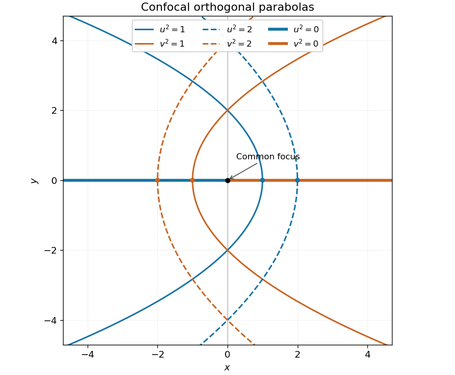
Signed coordinates. Take $u\ge 0$ and choose the sign of $v$ to agree with $y$ away from $y=0$. Then the Cartesian coordinates areEvery coordinate triple gives exactly one point. For $u>0$, $v$ and $y$ have the same sign. A fixed signed $v\ne 0$ selects the upper or lower half of its parabolic cylinder; the entire cylinder corresponds to fixed $v^2$. On the cut $u=0$, the two values $v=\pm \sqrt{-x}$ represent the same point of the negative $x$ half-axis. This boundary identification is unavoidable: there $y=0$ even when $v\ne 0$, so the sign prescription is understood by approaching from either side of the cut. The interior $u>0$ gives a unique coordinate chart off that half-axis.

Orthogonality and metric. Differentiate the position vector:The pairwise dot products vanish. Their lengths give the scale factors of orthogonal coordinates and hence the Riemannian metric:These are parabolic cylindrical coordinates. The differential calculation is regular for $u^2+v^2>0$; the $z$ axis is the coordinate singularity where the two planar tangent vectors vanish.

Laplacian. Put $h=2\sqrt{u^2+v^2}$. The physical components of the gradient of a $w$-independent scalar field are ${\varphi }_u/h,{\varphi }_v/h,0$. Applying the divergence formula cancels the two equal scale factors of orthogonal coordinates inside the derivatives:Therefore, away from the coordinate singularity,

Definitions. A group homomorphism $\phi :G_1\to G_2$ preserves multiplication, $\phi (xy)=\phi (x)\phi (y)$. A group isomorphism is a bijective group homomorphism. The kernel of a group homomorphism isPreserving multiplication implies $\phi (e_1)=e_2$ and $\phi (x^{-1})=\phi (x{)}^{-1}$: the first follows by cancelling $\phi (e_1)$ from its square, and the second follows by applying $\phi$ to $x{x}^{-1}=e_1$.

Kernel subgroup. The identity belongs to $K$. For $x,y\in K$, $\phi (xy)=e_2{e}_2=e_2$, so $xy\in K$. Also $\phi (x^{-1})=e_2^{-1}=e_2$, so $x^{-1}\in K$. Thus $\boxed{K\le G_1}$.

Normality. For $g\in G_1$ and $k\in K$,Hence every $gk{g}^{-1}$ is again in $K$, proving $\boxed{K⊴G_1}$. Applying the same statement with $g^{-1}$ gives equality $gK{g}^{-1}=K$, and therefore $gK=Kg$.

Group of cosets. Define the product on the left cosets byTo check that this does not depend on representatives, replace $a,b$ by $a{k}_1,b{k}_2$. Thenbecause normality puts $b^{-1}{k}_{1}b$ in $K$. Thus the product is well defined. It is associative because multiplication in $G_1$ is associative; its identity is $K=e_{1}K$, and the inverse of $aK$ is $a^{-1}K$. Consequently the cosets form the quotient group $\boxed{G_1/K}$.

The map $aK\mapsto \phi (a)$ is well defined and gives an isomorphism $G_1/K\cong \mathrm{im}\phi$. If the original mapping is onto $G_2$, this becomes $G_1/K\cong G_2$. No surjectivity is needed for the kernel of a group homomorphism to be a normal subgroup or for the quotient group to exist.

Cosets and Lagrange. A left coset is $gH=\{gh:h\in H\}$. The left cosets of a subgroup partition a group, each with $|H|$ elements. Lagrange's theorem states $\boxed{|G|=[G:H]|H|}$ for a finite group, so every subgroup order divides the group order.

The 64-element group. Work in the commutative ring $R=\mathbb{Z}/4\mathbb{Z}$, which has zero divisors. Denote the displayed lower triangular matrix by $A(a,b,c)$, where $a,b,c$ are its three entries below the diagonal. Direct matrix multiplication givesAll arithmetic is modulo four, so the set is closed. Associativity comes from matrix multiplication, the identity element is $A(0,0,0)$, andThe formula works in either multiplication order and requires no division. Hence these matrices form a group of order $\boxed{|G|=4^3=64}$. This is the lower triangular version of the Heisenberg group over a commutative ring.

The abelian subgroup. If $a=c$, write $h(a,b)=A(a,b,a)$. ThenThe identity is $h(0,0)$ and the inverse is $h(-a,a^2-b)$, proving an abelian subgroup. Its two independent entries give $\boxed{|H|=16}$ and $\boxed{[G:H]=4}$, in accordance with Lagrange's theorem. This is the abelian plane subgroup of the Heisenberg group modulo four.

More explicitly, $A(a,b,c)\mapsto a-c$ is a surjective group homomorphism to the additive group of $R$, with kernel $H$. The four left cosets are exactly the four sets with fixed $a-c=t$, $t=0,1,2,3$; representatives are $A(t,0,0)$. Thus $H$ is also a normal subgroup.

Matrices squaring to the identity. The product formula givesThe first and third coordinates vanish only when $a,c\in \{0,2\}$. Then $ca=0$ modulo four, so the middle coordinate vanishes exactly when $b\in \{0,2\}$. Therefore the complete set isIt is a subgroup: multiplying two such elements keeps all three entries even, and their cross term $cd$ vanishes modulo four, so the product simply adds the three even coordinates. The identity is included and each element is its own inverse. In fact $K$ is isomorphic to the direct product of groups $C_2\times C_2\times C_2$. The seven nonidentity elements are involutions.

Finally, the last subset in the PDF is defined by $a\ne 0\ne b$, with no restriction on $c$. It has $3\cdot 3\cdot 4=36$ elements, which cannot be a subgroup because $36$ does not divide $64$. It also excludes the identity element. Thus

General definitions. The Euler-Lagrange equation gives $m_i{\ddot{q}}_i+{\sum }_j{V}_{ij}{q}_j=0$. Write $M=\mathrm{diag}(m_i)$ and $K=(V_{ij})$. A normal mode has fixed displacement pattern $v$ and common time factor, $q(t)=vQ(t)$; its normal frequency satisfiesHere $\omega$ is angular frequency. A normal coordinate is the coefficient of one pattern in a complete modal expansion, so these coordinates decouple the equations. Since $M$ is positive definite, the change $z=M^{1/2}q$ turns the mode equation into the ordinary symmetric eigenvalue problem for $M^{-1/2}K{M}^{-1/2}$.

Three-mass equations. Let $x_1,x_2,x_3$ be horizontal displacements from the unstretched equilibrium, ordered left to right. The kinetic energy and potential energy areDifferentiating the potential energy givesThus $M=m\mathrm{diag}(1,2,3)$ and

Frequencies and patterns. Put $\lambda =m{\omega }^2/k$. Expansion of the generalized eigenvalue problem for small oscillations givesSolving at each root givesThe zero normal mode is uniform translation. In the lower nonzero mode, the central mass stays fixed, the two end masses move oppositely, and their unequal displacements balance both the end-mass momenta and the forces on the central mass. In the upper mode the end masses move together and the centre oppositely. Both vibrating modes leave the centre of mass fixed.

Orthogonality. Because $K$ is symmetric, two mode equations implyDistinct eigenvalues therefore give the mass-matrix orthogonality of normal modes:The Euclidean dot product need not vanish for unequal masses; for example $v_0^T{v}_1=-2$, while $v_0^{T}M{v}_1=m(-3+3)=0$. The modal squared norms are $6m,12m,12m$.

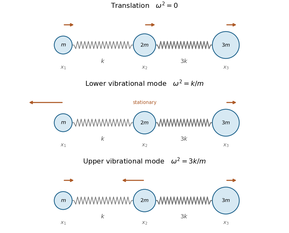
Normal coordinates. Expand $x=Q_0{v}_0+Q_1{v}_1+Q_3{v}_3$. Project using the mass-weighted inner product and divide by each modal norm to obtainFor example, the inverse equations are $x_1=Q_0-3Q_1+Q_3$, $x_2=Q_0-2Q_3$, $x_3=Q_0+Q_1+Q_3$. They reduce the energies toand henceThe first coordinate is the centre of mass and has free linear motion. Multiplying $Q_0,Q_1,Q_3$ by $\sqrt{6m},\sqrt{12m},\sqrt{12m}$ respectively gives mass-normalized normal coordinates if desired.

Tensor transformation. Under an orthogonal transformation $R$, the magnetic moment and magnetic field intensity have transformed components $M^{\prime }=RM$, $H^{\prime }=RH$ for a proper rotation. The physical relation $M=\chi H$ must retain its form, giving $RM={\chi }^{\prime }RH$, henceThis is precisely the law for a Cartesian second-rank tensor. Both magnetic quantities are axial vectors; under reflections they each acquire the same determinant sign, which cancels from the transformation of the magnetic susceptibility tensor.

Parallel directions. The condition $M=\lambda H$ is the eigenvalue equation $\chi H=\lambda H$. For the matrix in the paper, expansion of $\det (\chi -\lambda I)$ givesSolving the three resulting homogeneous systems givesThe three directions are mutually orthogonal. For the zero eigenvalue, the induced magnetic moment is zero: the proportionality equation still holds with factor zero, though there is then no nonzero moment direction to assign.

Energy extrema. The stipulated energy is $\mathcal{E}=H^T\chi H$. At fixed $H^{T}H=H_0^2>0$, a Lagrange multiplier calculation givesbecause $\chi$ is a real symmetric matrix. Thus all stationary directions are the eigenvectors, for which $M=\lambda H$. Equivalently write $H=q_0{e}_0+q_1{e}_1+q_6{e}_6$; thenThe Rayleigh quotient immediately givesThe intermediate direction $e_1$ is stationary with $\mathcal{E}=H_0^2$ but is not an extremum on the sphere. At the minimum $M=0$, so the precise extremum condition is proportionality, including a vanishing proportionality factor.

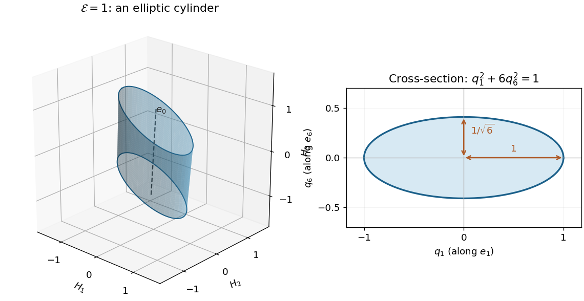
Constant-energy surface. In the original field components,For a fixed positive value $E$, $q_0$ is unrestricted and the cross-section satisfies $q_1^2/E+q_6^2/(E/6)=1$. The surface is therefore an elliptic cylinder, with axis along $(1,-1,2)$ and transverse semiaxes $\sqrt{E}$ along $e_1$ and $\sqrt{E/6}$ along $e_6$. This is an example of level sets of a positive semidefinite quadratic form. At $E=0$ the surface degenerates to the axis line; no negative-energy level exists.