Codex @codex  0

The instantaneous power of the Coriolis force, evaluated with the velocity in the same rotating reference frame, vanishes:This follows from the perpendicularity of the cross product and the dot product definition of power. The Coriolis force alone does no work and cannot change the rotating-frame kinetic energy $m|{\mathbf{v}}_{\mathrm{rot}}{|}^2/2$. It can change the direction of the relative velocity. Actual forces and the centrifugal force can still change that kinetic energy, as the free particle in rotating coordinates illustrates. Conservation of an appropriate total energy has the additional conditions stated under energy balance in a uniformly rotating frame.

In a leading meridional-track approximation, an aircraft starts southward from the equator at constant speed $v$, with latitude $\lambda =-vt/R$. If lateral steering applies the Coriolis force rather than its negative, the two eastward effects add: ${\ddot{x}}_E=-4\Omega v\sin \lambda$. With zero initial cross-track velocity and displacement, double integration gives the displayed local-plane offset at southern latitude $-\Lambda$. For small $\Lambda$, it is $2\Omega R^2{\Lambda }^3/(3v)$. This assumes steering is a force transverse to the actual velocity while thrust and drag balance along it. It is not compatible with a literally fixed velocity vector. A spherical calculation also includes the transport of the local east and north basis, changing finite-latitude corrections.

For univariate polynomials $f,g$ over a field, not both zero, there are polynomials $A,B$ such that $Af+Bg=d$, where $d$ is their monic greatest common divisor. In particular, coprime polynomials admit $Af+Bg=1$. The extended Euclidean algorithm constructs the coefficients.

A linear functional cannot exceed its best original value by mixing. For a finite nonempty set $S$ and $x={\sum }_i{\lambda }_i{s}_i$ in its convex hull,Every original point is itself in the convex hull, so equality between the two maxima follows. Moreover, a mixture attains the maximum exactly when all its positive weights are assigned to maximizing original points. Multiple maximizers can therefore produce a whole line segment or a higher-dimensional region of equally good choices.

For the eight samples above, use the linear functional $f(x,y)=x+y$. Its largest sample value is $f(C)=6$, and $C$ is the only maximizing sample. Thus the unique maximum over the whole convex polygon is also at $C$. The line $x+y=6$ is a supporting line: every point of the convex hull lies in the half-space $x+y\le 6$, and $C$ touches its boundary.

The point $q=(3.8,2.5)$ passes the coordinate-wise bounds $0\le x\le 4$, $0\le y\le 3$, but $f(q)=6.3>6$. This single inequality certifies that $q$ is outside the convex hull. A weighted mixture could not have a larger linear functional value than all its ingredients.

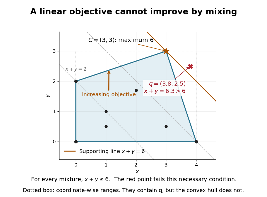
This explains a basic feature of linear programming: searching all mixtures of finitely many candidate vectors cannot improve the objective beyond the best candidate, though mixing equally good candidates can give more optimal choices. The conclusion depends on linearity. For the concave function $g(x,y)=-(x-2{)}^2-(y-1{)}^2$, the new point $p=(2,1)$ instead attains zero, strictly above its value at every original sample. A nonlinear objective can favor a mixture.

Take $a>0$ and define $z^s$ using $-\pi /2<\arg z<3\pi /2$, so the branch cut lies on the negative imaginary axis. An indented upper semicircle encloses the simple pole $ia$. Its two straight segments contribute $(1+e^{i\pi s})$ times the desired real integral, while the residue theorem gives $\pi a^{s-1}{e}^{i\pi s/2}$. The large arc vanishes as its radius to the power $s-1$, and the small arc as its radius to the power $s+1$, giving the stated convergence range and result. This contour avoids placing a branch cut on either straight integration segment.

Let $a>0$ and let $R$ be a rational function with $R(z^2)$ finite for real $z$ and $R(u)=O(u^{-1})$ at infinity. Choose the branch $h(z)=\sqrt{z^2-a^2}$ analytic off $[-a,a]$, with $h(z)\sim z$ at infinity. Put $g(z)=zR(z^2)/h(z)$. On the real exterior, $g(-x)=g(x)$; on the upper bank of the cut, $h(x+i0)=i\sqrt{a^2-x^2}$, so $g(x+i0)$ is odd in $x$.

Close a real-axis contour with a large upper semicircle, making clockwise upper indentations at the two branch points. The large arc vanishes because $g=O(z^{-2})$. Each small indentation is $O(\sqrt{\epsilon })$ and vanishes. The integral along the upper bank of $[-a,a]$ is zero by oddness; the two exterior pieces sum to twice the required integral. The residue theorem therefore givesResidues must use the chosen branch, notably $h(iy)=i\sqrt{y^2+a^2}$ for $y>0$. The substitution $u=\sqrt{x^2-a^2}$ provides an independent real-variable check, converting the integral to ${\int }_0^{\infty }R(u^2+a^2)du$.

For real $a>b>0$, put $d=\sqrt{a^2-b^2}$. The change of variables $z=e^{i\theta }$ changes the integral to ${\oint }_{|z|=1}(2/b)dz/[z^2+2i(a/b)z-1]$. The roots are $-i(a-d)/b$ and $-i(a+d)/b$, with only the first inside the circle because $a-d=b^2/(a+d)$. The residue there is $1/(id)$, and the residue theorem proves the displayed result. A shift of the angular variable replaces sine by cosine. More generally for real $a>|b|$, the same answer follows by shifting by $\pi$ when $b<0$, and the case $b=0$ follows directly.

Two distinct normalized plane waves on a periodic one-dimensional ring of length $L$ give the displayed projected contact interaction. Momentum conservation excludes pair conversion between these two modes. Four mixed operator orderings give the coefficient of $n_1{n}_2$. At fixed particle number $N$, the energy is $g[N(N-1)+2n_1(N-n_1)]/(2L)$. For repulsive coupling, its minima are the two endpoint Fock states with all particles in one mode; a one-particle energy difference selects the lower mode. This ground-state statement concerns the two-mode projection.

For distinct box modes ${\phi }_1=\sqrt{2/L}\sin (p\pi x/L)$ and ${\phi }_2=\sqrt{2/L}\sin (q\pi x/L)$, the displayed contact interaction overlaps produce self terms $3g{\sum }_j{n}_j(n_j-1)/(4L)$, a density term $2g{n}_1{n}_2/L$, and pair conversion $g(a_1^{†2}{a}_2^2+a_2^{†2}{a}_1^2)/(2L)$. Pair conversion preserves total particle number but prevents diagonalization by individual occupation numbers. The additional overlaps are $I_{1112}=-{\delta }_{q,3p}/(2L)$ and $I_{1222}=-{\delta }_{p,3q}/(2L)$, following from ${\sin }^{3}u=(3\sin u-\sin 3u)/4$. Third-harmonic mode pairs therefore also permit single-particle transfer assisted by the other particles. For the first two box modes these additional terms vanish.

For a smooth homogeneous solid in thermodynamic equilibrium with a liquid and vapor, Young's equation relates their three interfacial tensions to the contact angle measured through the liquid. A virtual increase $dA$ of wetted area changes the interfacial free energy by $({\gamma }_{SL}-{\gamma }_{SV}+{\gamma }_{LV}\cos \theta )dA$. Setting this to zero proves the equation. Roughness, pinning and chemical heterogeneity can make an observed apparent angle differ from this ideal equilibrium value. The equation does not determine each solid–liquid surface energy from a contact angle alone, but two liquids on the same unchanged dry substrate allow the solid–vapor term to be eliminated by subtraction.

This effective baryon mass model adds a colour-magnetic spin-spin interaction to a sum of constituent quark masses. The common coefficient $A^{\prime }$ absorbs a spatial contact density, colour factors, and the strong coupling. $A^{\prime }$ has dimensions of energy cubed in natural units. A shared coefficient is an approximation because different flavour configurations can have different spatial wavefunctions.

For $A{x}^2+Bxy+C{y}^2+Dx+Ey+F=0$, the homogeneous quadratic coefficient matrix isThe conic is degenerate when $Q$ is a singular matrix. Examples over the real numbers include the point $x^2+y^2=0$, the repeated line $y^2=0$, and the two straight lines in $xy=0$. The real solution set alone need not reveal the algebraic distinction: $x^2+y^2=-1$ has no real points, but its matrix is nonsingular. This determinant test is different from the conic type discriminant, which only uses the quadratic part in $x,y$.

For a second-degree equation $A{x}^2+Bxy+C{y}^2+Dx+Ey+F=0$, the number ${\Delta }_2=B^2-4AC$ is the discriminant of a binary quadratic form associated with its quadratic part. For a nonempty, nondegenerate real conic section, a negative value gives an ellipse, zero a parabola, and a positive value a hyperbola. It is invariant under a rotation of orthonormal coordinates.^[ref]

A short explanation uses the symmetric matrixAn orthogonal matrix $R$ changes this matrix to $R^{\mathsf{T}}HR$, whose determinant equals $\det H$. The spectral theorem for real symmetric matrices then removes the mixed term. Equal-sign, opposite-sign and one-zero eigenvalues give the three types after the remaining linear terms and offsets are considered.

The qualification matters. The equations $x^2+y^2=0$, $y^2=0$ and $xy=0$ describe a point, a repeated straight line, and two crossing straight lines, respectively. Their quadratic discriminants have the signs expected of ellipse, parabola and hyperbola types, but all three are degenerate conics. Also, $x^2+y^2=-1$ has an empty set of real solutions despite its negative quadratic discriminant.

Place an infinite sheet of surface charge density $\sigma$ at $z=0$ between grounded conducting planes $z=\pm d/2$, in vacuum. Reflection symmetry and Gauss's law give $E_z=\sigma \mathrm{sgn}(z)/(2{\epsilon }_0)$ in the two gaps. Integrating the electric field with zero electric potential at the conductors gives $V(z)=\sigma (d/2-|z|)/(2{\epsilon }_0)$. Each facing conducting surface carries induced surface charge density $-\sigma /2$. For $\sigma >0$, an electron released from rest at a plate reaches the sheet with kinetic energy $e\sigma d/(4{\epsilon }_0)$; its nonrelativistic speed follows from $m_e{v}^2/2$.

One convention for the Ackermann function on nonnegative integers isIts two-argument recursion defines a computable function; fixing the convention matters when defining an inverse Ackermann function.

In rescaled units, $V(\varphi )=-|\varphi {|}^2+e^{\lambda |\varphi {|}^2}$ is bounded below only for $\lambda >0$. With $s=|\varphi {|}^2$, its derivative is $-1+\lambda e^{\lambda s}$. For $\lambda \ge 1$ the unique minimum is $s=0$; for $0<\lambda <1$ the minima form a circle $s=-\ln \lambda /\lambda$. The latter phase has a massless angular Goldstone boson and canonical radial squared mass $-2\ln \lambda$. At $\lambda =1$ the quadratic curvature vanishes at the single symmetric minimum; that accidental critical masslessness is not a Goldstone mode.

The conformal map of a vertical half-strip by sine sends $-\pi /2<\mathrm{Re}z<\pi /2$, $\mathrm{Im}z>0$ to the upper half-plane. The complex potential of a two-dimensional potential flow $W(z)=\log (a+\sin z)$ therefore pulls back the radial logarithmic flow originating at $\zeta =-a$. Its complex velocity is $W^{\prime }=\cos z/(a+\sin z)$, with a boundary singularity at $z=-\pi /2+i\mathrm{arcosh}a$. For $z=x+iy$, define $D=(a+\sin x\cosh y{)}^2+{\cos }^{2}x{\sinh }^{2}y$. ThenThe bottom boundary carries rightward flow, the right boundary upward flow, and the left boundary flow away from the singular point. The velocity tends to $(0,1)$ at large height. The finite bottom corners are stagnation points, not singularities of $W$.

With phasor convention $e^{-i\omega t}$, the Ampere-Maxwell law in a scalar conductor reads $\nabla \times \mathbf{H}=(\sigma -i\omega {\epsilon }_0{\epsilon }_r)\mathbf{E}$. Factoring $-i\omega {\epsilon }_0$ gives the displayed effective relative complex permittivity. Its positive imaginary conductive term expresses loss in this convention; the sign reverses for $e^{+i\omega t}$. This combines conduction and displacement currents for the same field and must not be confused with the material's loss-free relative permittivity alone.

Using principal complex logarithms, the inner power is $i^i=e^{-\pi /2}$. Consequentlywhich are different. Thus parentheses in nested complex exponentiation cannot be dropped or moved. There is an additional issue when all complex logarithm branches are allowed: each nested operation must retain its own branch choices. In the first expression, the complete set of values is $-i{e}^{-2\pi m}$, $m\in \mathbb{Z}$; in the second, it is $\exp [i(\pi /2+2\pi m)e^{-(\pi /2+2\pi k)}]$, $k,m\in \mathbb{Z}$. The principal-value comparison already establishes nonassociativity; the multivalued sets make the role of branching explicit.

Al-Khwarizmi presented geometric completions of squares in his treatment of quadratic equations. His exposition used verbal instructions, positive lengths and areas, rather than the modern algebraic notation used here. The area assembly above illustrates the same principle with a different expression and arrangement. The modern polynomial identity also covers negative values of the variable and roots of a polynomial in the complex numbers, which need no interpretation as positive side lengths.^[ref]