
Forbidden beta decay 2026-10-18
A beta decay transition for which the leading lepton orbital term vanishes by the angular momentum or parity selection rules. The least contributing orbital order gives the name th forbidden. First-forbidden transitions change parity and can carry total lepton angular momentum ; second-forbidden transitions preserve parity and can carry , with Fermi-type contributions restricted to . Forbidden is suppression by higher powers of lepton momentum times nuclear size, rather than an absolute prohibition.
Comparative half-life 2026-10-18
The product of a dimensionless beta-decay statistical phase-space factor and the partial half-life for the transition. The tabulated normally means . Factoring out this approximate phase space dependence allows comparisons of nuclear weak matrix elements. Strong superallowed Fermi transitions have small ; forbidden beta decays generally have larger values, with nuclear-structure exceptions and overlaps between categories.
Fourier transform of the Bessel function J0 Created 2026-10-18 Updated 2026-10-20
With the Fourier transform convention , the regular order-zero Bessel function of the first kind has the tempered distribution transformThe density is integrable despite its endpoint singularities. Fourier inversion gives the equivalent integral representationThe second formula follows by and cancellation of the odd imaginary part. It is the standard real integral representation of .[ref]
Indeed, transforming the order-zero Bessel differential equation gives . Inside , its solutions are . The compactly supported choice also solves the equation as a distribution: rewrite it as , and observe that is continuous and zero at the two endpoints. Its distributional derivative has no endpoint Dirac delta terms. The inverse is regular at , and fixes .
The transformed equation alone also allows separate constants on and . Selecting the compactly supported density amounts to selecting the solution regular at the origin, rather than every possible singular solution of the Bessel differential equation.
Sturm-Liouville formulation with Bessel order as eigenvalue Created 2026-10-18 Updated 2026-10-20
For fixed , move the order term of the Bessel equation to the right: . The integrating factor for its leading differential expression is , giving the displayed Sturm-Liouville theory form with coefficient , potential , weight and eigenvalue . The origin is a singular endpoint. The integrating factor must be normalized from a positive reference point; its defining logarithmic integral cannot literally start at zero. Boundary conditions are needed before this differential identity becomes a specified self-adjoint spectral problem.
Berry curvature Created 2026-10-18 Updated 2026-11-05
The Berry curvature measures the local twisting of the quantum phase convention of a smoothly varying, nondegenerate energy eigenstate. For the Berry connection , it is the differential formChanging the state representative by changes by but leaves invariant. Thus the Berry connection depends on a phase convention, while the Berry curvature has convention-independent local content.
For a surface whose boundary is a closed parameter path, Stokes theorem expresses the Berry phase as the integral of the Berry curvature, provided the chosen patch is smooth on the surface. For a spin one-half aligned with a slowly turning magnetic field, the curvature yields a Berry phase equal to minus half the oriented solid angle for the positive-spin branch. The spectral gap must remain open; a quantum degeneracy can obstruct a single smooth choice over the whole surface.[ref]
Work by Bernhard Dobberstein 2026-10-18
Bell test Created 2026-10-18 Updated 2026-10-20
A Bell test compares experimental probabilities or expectation values with a Bell inequality. In a two-setting photon polarization test, each station chooses a polarizer orientation and records an outcome. A coincidence circuit identifies candidate pairs using an agreed timing rule. The choice of which trials enter the statistic is part of the experiment: correlations calculated only from detected pairs can differ from correlations of all emitted pairs. The Polarization CHSH count model separates ideal expectation values from this experimental selection problem.
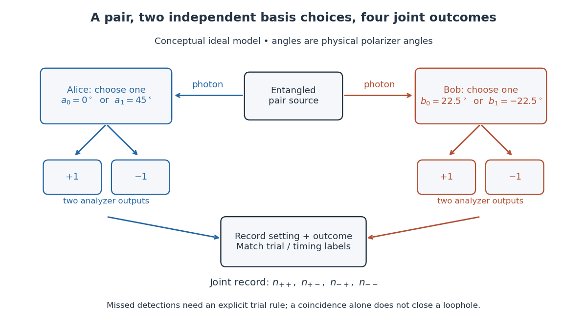
Two-setting polarization measurements and coincidence readout
. Conceptual apparatus for the ideal two-output model. The displayed angles belong to the worked CHSH example; they are not a reconstruction of a historical apparatus. Each station chooses one basis, then records either output. The coincidence record also needs a rule for missed detections. Details.
Reference blank 2026-10-18
A reference blank is the comparison sample used to establish the background response in a measurement. For absorbance, it contains matching solvent and other assay ingredients without the target absorbing chemical species; it sets the reference radiant power under matching cuvette and wavelength conditions.
Superconducting isotope effect 2026-10-18
The superconducting isotope effect is the dependence of the superconducting transition temperature on isotopic mass at fixed chemical composition. Its discovery in 1950 was a crucial clue that phonons participate in conventional superconductivity.[ref]
Electron-Phonon Interactions and Superconductivity by John Bardeen. p.55, isotope-effect discovery and its significance for the electron-phonon mechanism
The model prediction can be derived from two assumptions. For harmonic motion with a fixed restoring-force constant , a phonon frequency scales as . If the BCS dimensionless coupling is independent of , the weak coupling result then gives and . Changes in the effective interaction can change this exponent; it is not a universal law for every material exhibiting superconductivity. For a stipulated mass ratio , the ideal model predicts . This is an original scaling example, not a pair of measured transition temperatures.
BCS coherence length 2026-10-18
The clean isotropic weak-coupling BCS coherence length is conventionally , with Fermi velocity . It characterizes the spatial extent of pairing correlations.[ref]
The scale follows from the same spectral calculation. Linearizing the normal energy near the Fermi surface gives . The region therefore has radial width . Fourier analysis associates this width with a distance . This argument establishes the scale, not the conventional factor . A small superconducting energy gap consequently permits pairing correlations over many interparticle spacings.
BCS quasiparticle spectrum 2026-10-18
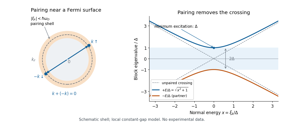
The BCS quasiparticle spectrum is the positive excitation energy obtained by diagonalizing the paired particle-hole block. Here the weak coupling shell model has : the minimum lies inside the pairing shell, and states outside it cost more. To derive it for a uniform isotropic real , measure the normal-state energy from the chemical potential, , and use the same sign convention as the BCS coherence factors:Its eigenvalues are , where . The positive is the cost of creating a quasiparticle above the BCS ground state. The lower branch is its particle-hole partner in this doubled matrix description, not an excitation that lowers the ground state energy without bound.
The location and value of the minimum follow directly:The unique minimum as a function of is , at the normal-state Fermi surface. On an isotropic three-dimensional Fermi surface it occurs for every direction of , rather than at a unique point of momentum space. Near that minimum,Farther away, when . For the illustrative example, a state at costs rather than the minimum .

Conservation of vorticity flux through a material surface Created 2026-10-18 Updated 2026-11-05
For smooth inviscid barotropic fluid with potential body forces, barotropic vorticity transport and give . Combine this with material surface element evolution to obtain . Integrating over a material surface proves the flux law. Its boundary must move with the fluid; flux through a fixed open surface is generally not conserved. By Stokes theorem the same statement is Kelvin's circulation theorem around the material boundary.
Near-axis radial velocity in incompressible axisymmetric flow Created 2026-10-18 Updated 2026-11-05
For a smooth axisymmetric flow, write near the axis. The incompressible flow condition is . Integrating radially and excluding a singular line source at the axis gives . The signed axial velocity is essential: specifying only its magnitude does not fix the sign of the radial velocity.
Macroautophagy Created 2026-10-18 Updated 2026-10-20
In macroautophagy, a portion of cytoplasm, potentially including an organelle, is enclosed in an autophagosome before delivery to a lysosome. Sequestration precedes digestion.[ref]
Transport from the Trans Golgi Network to Lysosomes. Molecular Biology of the Cell, 4th edition by Bruce Alberts and others; Multiple Pathways Deliver Materials to Lysosomes, autophagy paragraph and Figure 13-35
Attosecond streaking Created 2026-10-18 Updated 2026-10-20
Attosecond streaking uses a synchronized reference electric field to change a photoelectron's outgoing momentum. Scanning relative delay produces an energy-versus-delay distribution. A short emission interval samples only a small part of the reference cycle; a longer interval samples a range of kicks and can broaden or reshape the distribution.
For an explicit classical limit, use the electric dipole approximation and choose the magnetic vector potential along the detection axis with and . Neglect the residual ion's Coulomb force. An electron released at with mechanical momentum obeysIndeed, integrating from release to the end of the field gives the stated minus sign. The useful clock variable here is , rather than the instantaneous itself. If is nearly linear across a narrow emission window with temporal standard deviation , and initial momentum is sharp, thenThis local mapping fails near a zero of , where first-order timing sensitivity vanishes. A real inversion must include the incident bandwidth, initial photoelectron distribution, collection angles and target–field response.
For an original dimensionless example in atomic units, choose , and . Then and , compared with initial kinetic energy . Reversing gives : the shifts are asymmetric because of the term. A measurement that keeps only the term linear in would miss in both cases.
RABBITT measures adjacent harmonic spectral phases through two-photon photoionization. A weak delayed infrared reference opens two interfering paths to a shared photoelectron energy; the two-path attosecond phase reconstruction spells out the inference.
Isolated attosecond pulse 2026-10-18
An isolated attosecond pulse has one dominant short burst within the observation window, with any satellite emission quantified. A broad optical spectrum alone cannot distinguish one burst from several. Selecting a generation interval and an appropriate spectral band can suppress neighboring bursts, but the resulting temporal contrast must still be tested.
For a simple calculation independent of any apparatus, let , with two nonoverlapping copies of a short optical pulse. Its optical spectrum has intensityA satellite produces spectral fringes of angular spacing when the two bursts are coherent and resolved. For chosen field-amplitude ratio , the satellite/main energy ratio is , while fringe visibility is . Weak satellite energy can thus leave substantial fringes. Averaging an uncontrolled removes the interference term without removing the satellite: absence of fringes alone does not prove isolation.
Attosecond pulse train 2026-10-18
An attosecond pulse train contains repeated short optical pulses. For a group of odd multiples of a common driving frequency, the separation is half the driving period when the relative spectral phases recur. The construction resembles mode locking, but the participating components come from high harmonic generation, rather than separate resonant modes of a laser oscillator.
High harmonic generation Created 2026-10-18 Updated 2026-10-20
High harmonic generation converts an intense driving electric field into radiation at high integer multiples of its frequency. High harmonic generation in a gas is a process in nonlinear optics: an electron can leave a neutral target by tunnel ionization, gain kinetic energy in the driving electric field, and return to radiate upon recombination. This three-step picture is an approximate account of a probability amplitude for emission in quantum mechanics, not a measured path of one electron.[ref]
Generation and Measurement of Isolated Attosecond Light Pulses by Michael Hentschel. Generation and Measurement of Isolated Attosecond Light Pulses, slide 5: tunnelling, acceleration and return
Why odd multiples? In an ideal centrosymmetric gas driven by a single frequency, assume the radiating electric dipole moment satisfies , where is the driving period. Its Fourier series coefficient obeys , so every even coefficient vanishes. A finite envelope, an oriented target or an additional driving frequency can invalidate that symmetry argument. Producing many odd components also does not prove that their spectral phases form a short optical pulse.
The 1988 report involving Anne L'Huillier observed odd multiples of a driving wavelength in rare gases, reaching order 33 in argon. The unexpectedly slow fall of yield beyond the fifth order supplied a broad spectral plateau. A spectral observation alone did not establish the relative spectral phases needed for an attosecond pulse train.[ref]
Multiple-harmonic conversion of 1064 nm radiation in rare gases by M. Ferray and others. Multiple-harmonic conversion of 1064 nm radiation in rare gases, abstract
If a measured unattenuated reference rate includes the same additive background as subsequent measurements, then , where is signal alone. Substituting into an attenuation count model with an additive background gives . This automatically returns the measured reference at and tends to at strong attenuation. Adding directly to would count background twice at zero attenuation. A joint count likelihood can fit the reference and attenuated data with their separate exposure times, avoiding the need to regard the reference estimate as exact.
There are unlisted articles, also show them or only show them.