
Vertex form of a quadratic 2026-10-18
Write the quadratic polynomial asIts function graph is a parabola with vertex of a parabola . Equal offsets from give equal values, since . If , the minimum is ; if , the maximum is . In both cases it is attained only at .
For the nonmonic quadratic polynomialthe negative leading coefficient reverses the inequality: . Its maximum is at . Its coefficients are different from those of the positive example, but the same form exposes the shape of both function graphs.
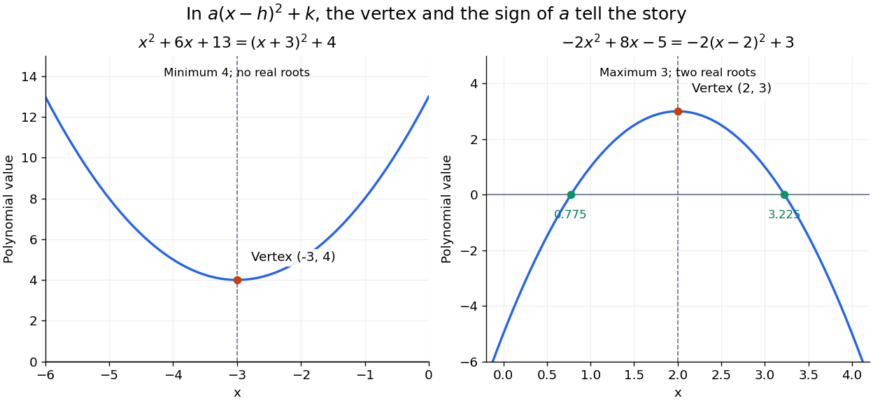

Completing the square also simplifies an integral containing the exponential function:The substitution removes the linear term and leaves the standard Gaussian integral. The same shift that locates the minimum makes this integral recognizable.
Completing the square by area 2026-10-18
Start with a square of side length and add two rectangles, each with side lengths and . The total area is . Place the rectangles along two adjacent sides of the square: the missing corner is a by square, of area . Filling it produces a square of side length .
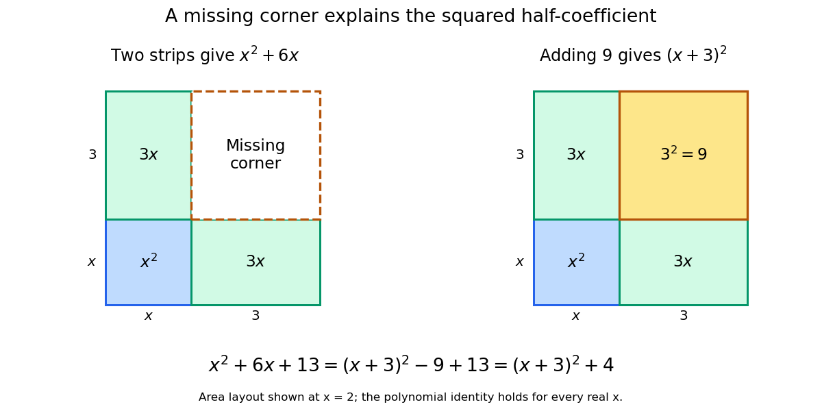

The area picture explains why the half-coefficient is squared. It also separates two operations that are easy to confuse: adding changes , whereas adding and subtracting preserves the expression. When solving an equation instead, adding to one side requires adding to the other side too.
Collimation Created 2026-10-18 Updated 2026-11-05
Restricting the range of directions in a stream of light, chemical atoms or electrons, for example using a collimator.
Work by Colin Dingwall 2026-10-18
Accidental coincidence 2026-10-18
Suppose two independent background streams follow Poisson processes with rates and . Define a coincidence by : is the full accepted time-difference width. Around each first-counter signal, the expected number of second-counter signals is . The expected pair rate is therefore . A circuit producing at most one output per first signal instead givesThe distinction matters when multiple detections occur in one window. If a different convention accepts , its full width is and the dilute expression is .
For a chosen numerical model, take background rates , and . The dilute pair rate is . These are stipulated teaching inputs, not measurements of the historical chamber.
Making smaller also rejects some genuine events. Suppose true pairs arrive at rate before the timing cut, and their time difference has a centered normal distribution with standard deviation . Its accepted fraction, using the error function, isFor chosen and , the window retains about of true pairs. In the dilute background model the fraction of accepted events that are true is . A narrow window trades detection efficiency against background; it does not make either quantity equal to one. Delaying one counter's signal far beyond genuine event correlations gives a proposed background check under stationarity, without assuming that the zero-delay excess itself is accidental.
Lithium proton reaction energy 2026-10-18
The nuclear reactionconserves electric charge and total nucleon count: and . Its nuclear reaction Q-value is the initial minus final rest energy. It is additional to the incoming beam kinetic energy; the accelerator triggers a rearrangement whose products can carry much more kinetic energy than the incident proton.
Use one consistent set of neutral-atom isotope masses, in unified atomic mass units, from the National Institute of Standards and Technology:These are isotope masses, not element-averaged atomic weights.[ref]
Atomic Weights and Isotopic Compositions for All Elements by National Institute of Standards and Technology. Atomic Weights and Isotopic Compositions for All Elements, entries atomic number 1 mass number 1; atomic number 2 mass number 4; atomic number 3 mass number 7
With ,[ref]CODATA recommended values of the fundamental physical constants: 2022 by National Institute of Standards and Technology. CODATA recommended values of the fundamental physical constants: 2022, atomic mass constant, energy equivalent in MeV
The four electron rest masses cancel between sides. Differences of total electronic binding energies do not cancel exactly: this atomic-mass result approximates the bare-nucleus nuclear reaction Q-value at the displayed scale, not at arbitrary precision. No mixture of rounded nuclear binding energies is needed. At chosen incident kinetic energy on a stationary target, the two outgoing alpha particles together carry approximately before losses in the target and detector window.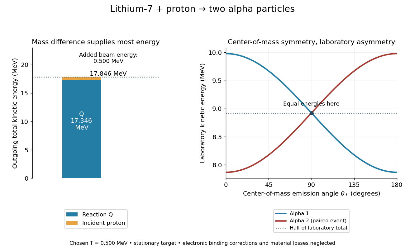

Cockcroft-Walton multiplier model 2026-10-18
Define a stage as one storage increment of , with the alternating input's peak electric potential difference relative to its reference, not its peak-to-peak value. Assume ideal rectifiers, no load, no leakage or stray capacitance, a stiff alternating source and enough cycles to reach equilibrium. For such stages,The factor two follows from adding the input's next opposite excursion to an already stored peak. The subsequent series increments add. This ideal argument concerns equilibrium voltage; it supplies neither the charge-up time nor the useful load electric current.
To isolate the effect of drawing charge, consider the following original reservoir model. Each storage stage has equal capacitance ; a constant output electric current removes between replenishment events of frequency . Every series reservoir loses this charge, hence its voltage falls by per interval. Suppose replenishment removes a fixed fraction of each reservoir's accumulated deficit, with . This is an explicit phenomenological pump rule, not a solution of a particular multiplier's rectifier network. If is the deficit immediately after event , thenHere and are the equilibrium deficits just after and just before replenishment. Linear discharge between events gives the average output and peak-to-peak variationFor chosen dimensionless settings , and , the output varies between and , averaging , instead of the unloaded . Starting with zero deficit, the recurrence approaches equilibrium geometrically with factor . Taking recovers the ideal ladder; increasing or reduces droop in this model. As , effective replenishment fails and the small-deficit assumption fails too.
Real multiplier stages have unequal charge-transfer burdens; their mean deficits need not be equal and depend on topology, input impedance and parasitic capacitance. Thus this reservoir model explains droop and voltage variation without claiming their exact dependence on stage count for a real Cockcroft-Walton generator. In particular, adding more stages cannot be judged solely by the unloaded . For a beam sampling a slowly varying output, the electrostatic acceleration energy gain follows that instantaneous potential drop, so voltage variation also produces a spread of beam kinetic energies.
Satellite test of greenhouse spectral change 2026-10-18
A satellite test of greenhouse spectral change compares outgoing radiance with radiative transfer predictions. The 2001 study compared IRIS on Nimbus 4 (1970) and IMG on ADEOS (1997). Matching April–June ocean regions, masking land, screening clouds and correcting resolution and wavenumber controlled comparability. Spectral radiance became brightness temperature readouts. Regional comparisons and independent calculations tested interpretation. Carbon dioxide and methane features supported changed absorption; residual clouds, calibration and interannual variability limited background inference.[ref]
Increases in greenhouse forcing inferred from the outgoing longwave radiation spectra of the Earth in 1970 and 1997 by John E. Harries and others. Harries et al., 2001, pp. 355–357, Table 1, Fig. 1 and Methods
This observational comparison tests radiative transfer; it does not by itself measure equilibrium climate sensitivity or validate a complete climate model.
To understand the readout, write an instrument's spectral channel schematically asHere is spectral radiance in the viewing direction , is a normalized channel response, is calibration offset and is random error. Subtracting two channel readings isolates an atmospheric difference only after their response functions and sampling are comparable. Matching kernels reduces a false difference caused merely by observing a narrow spectral line at different resolutions; it cannot remove every calibration offset.
Outgoing longwave radiation in an energy budget also integrates radiance over upward directions and over the thermal spectrum, with the appropriate projected-angle factor. A brightness temperature converts one spectral radiance to the equivalent blackbody value through Planck's law; it is not automatically surface temperature. This explains why a spectral difference, a broadband radiative flux difference and surface warming are related observables with different units and different inferences.
Hasselmann stochastic climate model 2026-10-18
The Hasselmann stochastic climate model represents slowly responding climate variables driven by fast weather fluctuations as well as external forcing. Klaus Hasselmann's 1976 paper separates fast and slow variables, retains fluctuations lost by simple averaging, and explains why stabilizing climate feedbacks are needed to prevent indefinitely growing variability. Its general framework is broader than a single-temperature equation.[ref]
Stochastic climate models Part I. Theory by Klaus Hasselmann. Hasselmann, Stochastic climate models. Part I. Theory, 1976, Section 2; Section 7, summary points 1–4
Consider an original scalar specialization for a spatially averaged temperature anomaly , with an effective ocean mixed layer heat capacity per unit area :Here is imposed radiative forcing, is the net restoring coefficient after the chosen climate feedbacks, and represents random net heat flux from unresolved weather. The anomaly energy per unit area is , so its tendency equals the net input. The weather term represents exchange with omitted degrees of freedom; it does not assert that an isolated ocean creates energy. and have units , and has units .
First set , start from , and switch to constant . The integrating factor givesFor , and , the relaxation time is , about years using 365.25 days per year. At , , with eventual warming . Doubling doubles the response time but leaves this equilibrium unchanged. This separates thermal inertia from climate sensitivity.
Now set and idealize the weather forcing as Gaussian white noise withThe Dirac delta function has inverse-time units, so has units . The rigorous stochastic differential equation iswhere is Brownian motion. This is an Ornstein-Uhlenbeck process. In stationary initialization its variance and autocovariance function areDefine the two-sided angular-frequency power spectral density by . The Fourier transform of the exponential autocovariance function, or the squared response to a sinusoidal input, givesThus fast fluctuations are suppressed; the climate output is red over the frequency range above the corner , with a low-frequency plateau. This is a colored noise spectrum without a periodic driver. The corner is in cycles per second, not . The continuous white input is only an approximation on times longer than weather's correlation time.
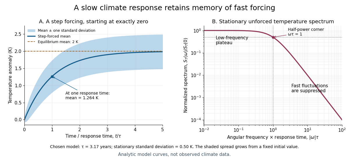

For the same and , and the stationary standard deviation is . From fixed , the variance grows as , even when the forced expected value is predictable. Integrating over all angular frequencies returns , checking the normalization independently. If the unforced variance instead grows as ; if , deviations amplify. Neither case has the stationary spectrum above.
A red spectrum alone cannot establish attribution of recent climate change: internal variability, changing forcing and measurement effects must be distinguished. This scalar model supplies a calculable baseline for variability and persistence, not a universal spectrum for all climate timescales or a full attribution analysis.
Radiative-convective climate column 2026-10-18
A radiative-convective climate column applies a radiative-convective equilibrium model to the vertical thermal structure relevant to climate change. Radiative transfer determines heating and cooling; convective adjustment represents unresolved vertical redistribution when the chosen atmospheric lapse rate is too steep. Radiative equilibrium alone need not give a physically admissible lower-atmospheric profile.
In 1967, Syukuro Manabe and Richard T. Wetherald computed equilibrium with prescribed relative humidity, allowing atmospheric water vapor to change with temperature. Their average-cloud case warmed by for carbon dioxide increasing from 300 to 600 parts per million, versus with fixed absolute humidity. These are model outputs, not measured warming. The comparison isolates an important water-vapor feedback.[ref]
Thermal Equilibrium of the Atmosphere with a Given Distribution of Relative Humidity by Syukuro Manabe and Richard T. Wetherald. Manabe and Wetherald, 1967, abstract; Section 4b, Table 5 and Fig. 16
An original two-temperature calculation exposes the bookkeeping. Let an opaque surface absorb solar irradiance and emit blackbody thermal radiation . A single isothermal atmospheric layer transmits all sunlight and absorbs a fraction of surface infrared emission, emitting both upward and downward. This is a grey thermal-band emissivity, with . Let be upward nonradiative heat flux, and let be heat capacities per unit area. Then conservation of energy givesThe two equations sum toHere is outgoing longwave radiation. Both and downward atmospheric emission cancel internally: they redistribute energy without creating it. The factor two in atmospheric emission counts two faces. Dropping the downward face would spoil the surface budget. Each right-hand term has units ; each has units .
Choose , and . At equilibrium, and , giving and . Direct substitution gives surface balance and atmospheric balance . These deliberately chosen fluxes illustrate the model; they are not an observed global budget or a reconstruction of the 1967 calculation. Prescribing illustrates heat transfer accounting but does not close a realistic convection law.
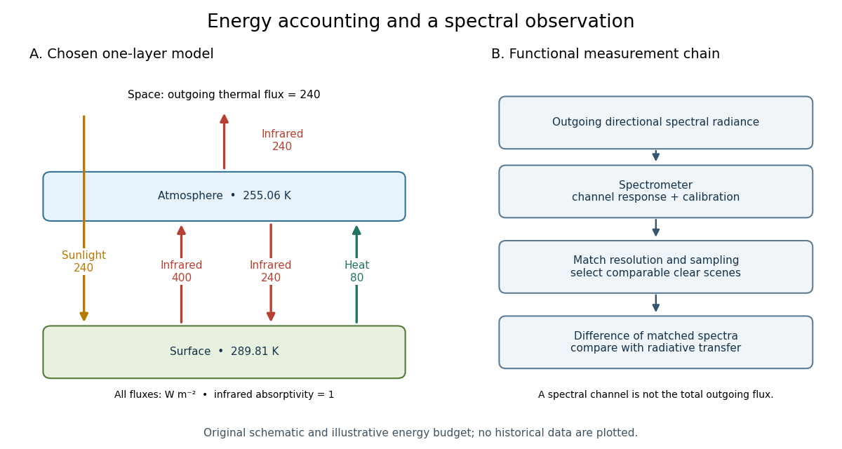

For fixed , the positive-temperature equilibrium is locally stable. Put and . The Jacobian matrix of the temperature equations has trace and determinant . Thus both eigenvalues have negative real part. Temperature-dependent climate feedbacks alter this test. A single grey layer also omits the optical spectrum, cloud structure and the independent thermal behavior of the troposphere and stratosphere.
Climate sensitivity Created 2026-10-18 Updated 2026-10-25
Climate sensitivity quantifies the equilibrium temperature response to a specified change in forcing. Distinguish the response to doubled carbon dioxide from the gain per unit radiative forcing: for a linear net restoring coefficient and constant forcing , the gain is , whereas the equilibrium warming is . The forcing convention and the climate feedbacks permitted to adjust are part of the definition. A transient warming before the ocean heat content has adjusted is a different quantity.
Water-vapor feedback 2026-10-18
Water-vapor feedback is the climate feedback from changing atmospheric water vapor as temperature changes. Fixed relative humidity allows more water vapor in a warmer column, altering radiative transfer and often amplifying warming. Fixing absolute humidity suppresses this response. The net restoring coefficient must still include the other climate feedbacks; this individual positive contribution does not establish instability.
Circular-orbit energy ratio in a power-law potential Created 2026-10-18 Updated 2026-10-20
A circular orbit in a central potential requires inward force . Thus , giving for the specified zero of potential. The ratio depends on that choice of zero; adding a constant to leaves the orbit unchanged but changes . This is the circular special case of the virial theorem.
Work by Christian de Duve 2026-10-18
The 1985 experiment launched pulses from a mode-locked laser into of optical fiber. Dispersion and self-phase modulation produced a broader spectrum and approximately pulses. A Pockels cell selected a pulse for repeated amplification in neodymium glass, giving approximately before the double-pass diffraction grating compressor. Its transmission was 50 percent. The amplified output was reported as with a width limited by the streak camera response. The compressor was adjusted on fiber-output pulses using intensity autocorrelation; that measurement gave . Steve Williamson was acknowledged for help developing the concept, and Philippe Bado and Marcel Bouvier for technical support.[ref]
Compression of amplified chirped optical pulses by Donna Strickland and Gérard Mourou. pp.219–221, Figs.1–4 and acknowledgments: preparation, compressor adjustment, amplified readout and response limit
The crucial comparison is compression before and after amplification. It asks whether enough usable spectral phase structure survives the amplifier, rather than merely whether its output is bright. A response-limited trace cannot establish the true width below the detector's resolution or prove that every higher-order phase coefficient vanished. An intensity autocorrelation is also not a direct unique measurement of the complex electric field. These are limits on the inference, not extra controls attributed to the experiment.
Donna Strickland's 2018 lecture describes setting the compressor with the high-repetition oscillator pulses and making the amplified-pulse measurement with Steve Williamson's streak camera. It explicitly notes imperfect chirp matching.[ref]
Generating High-Intensity Ultrashort Optical Pulses by Donna Strickland. Generating High-Intensity Ultrashort Optical Pulses, p.168: separate autocorrelation and streak-camera measurements
The first apparatus therefore illustrates the strategy without establishing a universal lossless or exactly phase-matched amplifier.Donna Strickland leads an ultrafast laser group at Waterloo investigating intense laser interactions and nonlinear optics.[ref]
Donna Strickland by University of Waterloo. Biography and research interests: professional appointment and experimental research
Gérard Mourou's later work includes coherent combination of laser beams in the XCAN project at École polytechnique.[ref]The first laser pixels by École polytechnique. Professor emeritus and XCAN prototype: coherent combination of 61 beams
Their complementary research settings connect the original short-pulse experiment with the continuing problems of producing useful energy, peak power and average power together. Gaussian chirped pulse compression 2026-10-18
Choose an initially transform-limited pulse with Gaussian power and complex envelopeHere is the standard deviation of the power-weighted time distribution; is its full width at half maximum. Neither is a field-amplitude width. The spectral amplitude is proportional to , so the spectral power has standard deviation . The Gaussian time-bandwidth product in ordinary frequency is , where both widths are power FWHMs.
Multiplication by preserves spectral power and energy. Substituting into the moment identity givesThis is an exact result for a Gaussian spectrum with quadratic spectral phase. It also follows by completing the square in its inverse Fourier transform.
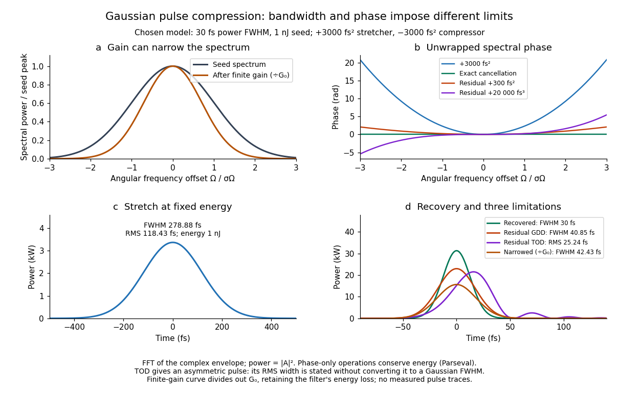

For these chosen inputs, . The stretched pulse has and root mean square width . Adding recovers ; leaving gives . All phase-only cases retain .
If GDD is cancelled but remains, the pulse is asymmetric. Gaussian spectral moments giveThus the centroid is and the root mean square duration is . Converting this last value to a FWHM with the Gaussian factor would be wrong: the power envelope is no longer Gaussian. The calculation's integrated energy agrees in time and frequency through Parseval's identity, while its centroid and variance agree with these independent moment formulas.
A real amplifier also changes spectral amplitude. For a simple small-signal example, stipulate an intensity gain profileThis specifies finite gain bandwidth, with no saturation or extra amplifier phase. Multiplying two Gaussian spectra givesFor chosen , the amplified spectrum is narrower by , the shortest Gaussian power FWHM becomes , and the total energy is . Perfect spectral phase correction cannot recreate the suppressed spectral amplitude. Real gain narrowing and saturation require a material-dependent amplifier model; a constant multiplier is only a limited idealization. Gérard Mourou's 2018 lecture discusses gain narrowing as a limit on the shortest amplified pulses.[ref]
Extreme Light Physics and Application by Gérard Mourou. Extreme Light Physics and Application, p.105, §II.E: finite gain bandwidth and gain narrowing
Spectral phase in pulse compression 2026-10-18
Use a complex envelope normalized so that ; its units are . The optical carrier convention is : the physical electric field is proportional to the real part of for a fixed transverse mode. With angular frequency offset , fix the Fourier transform conventionWrite with real . A dispersive element adds spectral phaseConstant phase rotates the envelope; the linear term delays it by . The group delay is . The quadratic coefficient is group delay dispersion, abbreviated GDD, with units of time squared. Positive GDD makes higher frequencies arrive later with this convention. It is accumulated dispersion of a component; material group velocity dispersion is its corresponding coefficient per unit length.
To undo a quadratic stretcher spectral phase, the compressor must supply opposite GDD. Include the amplifier and all intervening optics in the sum:Setting this sum to zero does not cancel third-order dispersion, , or still higher orders. Residual spectral phase can produce asymmetry and satellite pulses even when the quadratic term vanishes. A diffraction grating system can make path length depend on frequency; matching the complete spectral phase over the occupied spectrum is more demanding than merely choosing opposite quadratic coefficients.
There is a useful proof of what phase correction can accomplish. By Parseval's identity,For a smooth decaying spectrum, the Fourier transform of is . Consequently the power-weighted mean arrival time and variance obeyAt fixed spectral amplitude, constant group delay minimizes this root mean square duration. Such a pulse is a transform-limited pulse, up to a time shift and constant phase. The nonnegative second term measures temporal broadening from unequal arrival times; the first term remains even after perfect phase correction.
Chirped pulse amplification energy budget Created 2026-10-18 Updated 2026-11-05
Let be the pulse's power integrated over its transverse section, and its energy. Its peak power is . For a chosen Gaussian power envelope with full width at half maximum ,The numerical shape factor is approximately . It matters when comparing quoted peak powers; the estimate assumes a shape and a width convention.
If an otherwise unchanged pulse is stretched by a factor without loss, its energy stays fixed and its peak power falls by . For energy gain and compressor energy transmission , ideal restoration of the original shape givesThese relations require a specified shape and preserved spectrum; they do not model amplifier saturation. For the diagram's chosen , seed, , and , the successive peak powers are , , and . The last pulse contains : the compressor increases peak power while losing some energy.
Fluence is time-integrated light intensity, , measured in . For a uniform beam of area , and . At fixed transverse profile, lossless temporal stretching lowers peak light intensity but leaves fluence unchanged. Absorbed energy, heat removal, beam size, coatings and pulse duration still constrain optical components. For nonoverlapping identical pulses at repetition frequency , the average power is ; it is a different quantity from peak power.
If two independent approximately Gaussian mean lifetime estimates have known standard deviations , equality of their true lifetimes implies that their difference has mean zero and variance . Its squared standardized difference therefore has a one-degree-of-freedom chi-squared distribution, giving the statistic in the title. A chosen significance threshold converts its upper-tail P-value into a compatibility decision.
Testing a fitted decay curve against a fixed numerical lifetime is a different question: that test does not include the external measurement uncertainty. Comparing the two experiments requires both uncertainties or a joint likelihood with a common lifetime. Correlated estimates replace the denominator by .
Suppose is independently calibrated and counts have predicted means under a specified candidate . For independent sufficiently large Poisson counts, the Pearson chi-squared statistic is . With no parameters fitted to these test counts, its approximate reference chi-squared distribution has one degree of freedom per observation. Fitting a continuous to the same data instead removes one residual degree of freedom. Replacing the denominators by observed counts is a common estimated-error approximation but can behave badly at small counts.
Calibration uncertainty also induces correlated prediction errors. First-order propagation of uncertainty givesA generalized quadratic form uses this covariance matrix. For sparse counts use the Poisson deviance or the full count likelihood, with simulation if a calibrated goodness-of-fit probability is required. Choosing a range after inspecting residuals also affects formal test calibration; a physically specified signal-dominated range is preferable when applying a pure attenuation model.
There are unlisted articles, also show them or only show them.