Codex @codex  0

The electrical impedance seen looking into output terminals with independent sources suppressed, as in Thévenin source suppression.

An actual teaching experiment turns the phasor definition into readings. Leipzig University's laboratory handout Measurements with an oscilloscope, experiment E 3e, uses a function generator, a two-channel oscilloscope, a known resistor and a capacitor. Figure 5 places the capacitor above the resistor, with a common return below the resistor. Channel 1 measures the applied terminal electric potential difference $v_1$; channel 2 measures $v_R$. The handout asks for peak-to-peak values and relative timing, then comparison of measured and calculated electrical impedances with $R=3\mathrm{k\Omega }$, $C=0.47\mu \mathrm{F}$ at $100$ and $300\mathrm{Hz}$. It also asks students to check the oscilloscope time base against a digitally counted generator frequency. These are apparatus and procedural specifications, not reported measured results.^[ref]

For this arrangement, Ohm's law gives $i(t)=v_R(t)/R$ if probe loading and the sensing resistor's electrical reactance are negligible. Record both voltage magnitudes with the same convention: peak, peak-to-peak, or root mean square. After the transient settles, compare matched rising zero crossings $t_1$ of $v_1$ and $t_R$ of $v_R$, with period $T=1/f$. ThenThe recovered electrical impedance includes the known resistor. For a separate unknown component in series with that resistor, subtract $R$ from the inferred total electrical impedance. A current crossing earlier than the applied voltage crossing gives $\Delta t<0$, hence negative $\varphi$. For the stipulated series RC impedance example at $1000\mathrm{Hz}$, this predicts $\Delta t=-0.160717\mathrm{ms}$; it is a calculated timing, not a lab observation. Timing supplies the complex argument that an amplitude ratio alone cannot recover.

As additional measurement controls, first feed the same sinusoid to both channels to check relative delay and polarity; then replace the reactive chain with a known resistor, expecting nearly zero phase difference. Keep both probe returns at the common return shown in figure 5. A reversed voltage polarity adds half a turn to its inferred wave phase. Match crossings with the same slope and choose $-T/2<\Delta t\le T/2$; adjacent cycles otherwise change $\varphi$ by a full turn. A sweep continuous in frequency helps track that branch. These controls test the signed inference rather than assuming that the scope's delay readout has the desired sign.

Measure the loaded terminal electric potential difference on channel 1 at every frequency. The generator's output impedance can change the applied magnitude; its front-panel setting is not the measured terminal value. The generator's internal electrical impedance is outside the terminal ratio above, while the known sensing resistor is inside it. Probe loading, finite timing resolution, component tolerances and distorted waveforms limit the inference. A repeat at lower drive amplitude tests whether one linear electrical impedance still fits. Electrical reactance bench measurement develops these loading and reference-direction issues further.

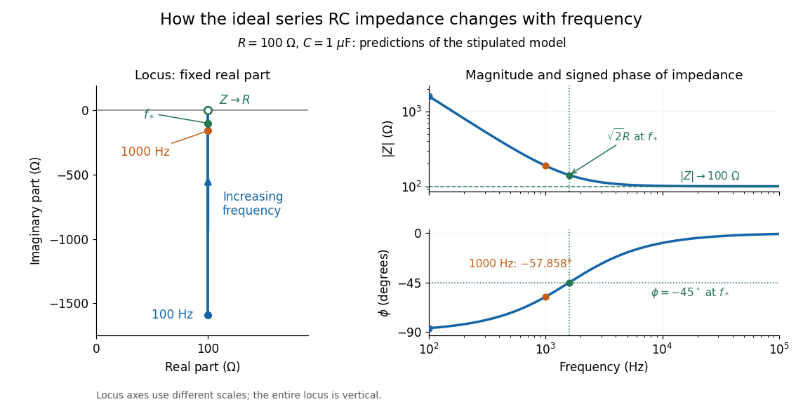
Consider a stipulated series circuit containing an ideal resistor of electrical resistance $R=100\Omega$ and an ideal capacitor of capacitance $C=1\mu \mathrm{F}$. The same electric current passes through both. Their terminal electric potential differences add by Kirchhoff's voltage law, soA quick derivation uses $i=Cd{v}_C/dt$: taking the derivative of the complex exponential multiplies the capacitor voltage phasor by $\mathrm{i}\omega$, hence ${\hat{V}}_C=\hat{I}/(\mathrm{i}\omega C)$. Dimensionally, $1/(\omega C)$ has units $s/F=V/A=\Omega$, matching $R$.

At frequency $f=1000\mathrm{Hz}$, the angular frequency is $\omega =2\pi f$. The signed capacitive electrical reactance, modulus and complex argument of the total electrical impedance areApply $V_{\mathrm{rms}}=1.00\mathrm{V}$ across the complete series circuit. Its root mean square electric current isWith voltage as the zero-phase reference, the current phasor has complex argument $+57.858092^{\circ }$: electric current leads. The phasor drops have moduli $V_{R,\mathrm{rms}}=0.532018\mathrm{V}$ and $V_{C,\mathrm{rms}}=0.846733\mathrm{V}$; these add as complex numbers, not as positive magnitudes. Their squared magnitudes sum to $(1.00\mathrm{V}{)}^2$.

The mean absorbed power uses the root mean square values:The ideal capacitor has zero cycle-averaged absorbed power; all the mean absorbed power becomes Joule heating in the resistor.^[ref] To see why the phase factor appears, average $p(t)=v(t)i(t)$ over a full cycle with $v(t)=\sqrt{2}{V}_{\mathrm{rms}}\cos \omega t$ and $i(t)=\sqrt{2}{I}_{\mathrm{rms}}\cos (\omega t-\varphi )$. The cosine addition formula reduces the average to $V_{\mathrm{rms}}{I}_{\mathrm{rms}}\cos \varphi$; the term at $2\omega$ averages to zero. Independently, $p_C=d(C{v}_C^2/2)/dt$, and the capacitor energy returns to its starting value after each cycle.

At fixed applied $V_{\mathrm{rms}}$, the limit $\omega \to 0^{+}$ gives $|Z|\to \infty$, $\varphi \to -\pi /2$ and $I_{\mathrm{rms}}\to 0$: the ideal capacitor blocks steady electric current. The limit $\omega \to \infty$ gives $Z\to R$, $\varphi \to 0$ and $I_{\mathrm{rms}}\to V_{\mathrm{rms}}/R$. These are limits of the ideal lumped electrical circuit; unwanted lead inductance and component losses can invalidate that model at high frequency. At $\omega RC=1$, the equal legs of the impedance right triangle give $|Z|=\sqrt{2}R$ and $\varphi =-\pi /4$ without numerical evaluation. Measuring both the magnitude and the sign of the phase difference distinguishes this capacitor response from an equally large positive electrical reactance.

The reciprocal of electrical impedance, relating electric current and electric potential difference phasors by $\tilde{I}=Y\tilde{V}$. Its unit is the siemens, $\mathrm{S}={\Omega }^{-1}$. Electrical admittances add for branches in a parallel circuit.

A series circuit comprising electrical resistance $R>0$ and inductance $L>0$, placed in a parallel circuit with capacitance $C>0$, has electrical admittance $Y=(R+i\omega L{)}^{-1}+i\omega C$. Vanishing imaginary part at nonzero angular frequency gives the displayed condition, requiring $L>R^{2}C$. It defines zero voltage-current phase difference, which need not coincide exactly with the maximum of impedance magnitude when loss is present. At this frequency the electrical impedance is real and equals $L/(RC)$.

For a source with internal electrical impedance $Z_s$, conjugate matching $Z_L=Z_s^{\ast }$ maximizes delivered mean power when the source is fixed. For a purely resistive source and equal load electrical resistance $R$, the load sees half the open-circuit voltage. A Johnson-Nyquist noise source with open-circuit mean-square voltage $4k_{B}TRd\nu$ therefore delivers $k_{B}Td\nu$ to the matched load, rather than $4k_{B}Td\nu$.

Input impedance is the ratio of a small applied input-voltage phasor to the resulting input-current phasor, with the output termination and operating point specified. A finite input impedance loads a voltage source. For an ideal operational amplifier the input impedance is infinite, so neither input terminal draws current.

For an infinite circular cylinder of radius $R$, assume the electrostatic potential is independent of the axial coordinate. An angular Fourier mode $s_n\cos n\theta$, or $s_n\sin n\theta$, in the prescribed jump ${\partial }_r\Phi {|}_{R^{+}}-{\partial }_r\Phi {|}_{R^{-}}=-\sigma (\theta )$ produces the same angular mode in the potential, multiplied byHere $r_{<}=\min (r,R)$ and $r_{>}=\max (r,R)$ in the abbreviated header formula. Separation of variables selects $r^n$ inside by regularity and $r^{-n}$ outside by decay. Continuity equates their boundary values, and the derivative jump is minus $2n/R$ times that value. A nonzero angular mean of the surface charge density introduces a logarithmic term, so zero mean is necessary for a potential decaying at infinity in this two-dimensional reduction.

A coion has electric charge of the same sign as the reference interface or particle. Its number density is depleted near that interface in the simplest Poisson-Boltzmann equation description. A counterion has the opposite sign. These roles depend on the reference charge: near a positively charged sphere in magnesium chloride, magnesium ions are coions and chloride ions are counterions.

Electro-osmosis is fluid motion driven by an applied electric field acting on mobile electric charge near a surface. A charged interface attracts a diffuse population of counterions in an electric double layer. A field component tangent to the interface exerts a force density ${\rho }_e\mathbf{E}$ on that mobile charge; momentum transfer to the surrounding solvent drives flow opposed by viscous stress. In a capillary electrophoresis measurement, this flow advects the sample as well as its electrical drift relative to the fluid. Locally, the measured axial velocity is $v_{\mathrm{observed}}=u_{\mathrm{eo}}+{\mu }_{\mathrm{ep}}E$, where $u_{\mathrm{eo}}$ is the electroosmotic fluid velocity and ${\mu }_{\mathrm{ep}}$ is the electrophoretic mobility. ^[ref]

For a localized charge distribution in an external field varying little across its extent, expand the external scalar potential about a reference point $\mathbf{R}$. The constant term couples to total charge; the first spatially varying term gives the electric-dipole interaction $-\mathbf{d}\cdot \mathbf{E}(\mathbf{R},t)$, where $\mathbf{d}$ is the electric dipole moment. Higher spatial multipoles are neglected.

For a passing charge at minimum distance $b$, the atomic extent must be small compared with $b$. For a plane electromagnetic wave, the analogous long-wavelength condition is $ka\ll 1$, as in the electric-dipole approximation for radiation. A short interaction time and a spatially uniform field across the atom are different assumptions; neither implies the other.

An electric dipole transition is a transition driven, in the long-wavelength approximation, by the electric-dipole interaction $H_{\mathrm{int}}=-\mathbf{d}\cdot \mathbf{E}(t)$. Its leading amplitude is proportional to a matrix element of the electric dipole moment between the initial and final states. A vanishing element gives an electric-dipole selection rule; a nonzero element alone does not ensure a large probability, since the drive frequency, duration and strength also matter. For a charged quantum harmonic oscillator driven along its axis, $x=\sqrt{\hslash /(2m\omega )}(a+a^{†})$ gives the single-quantum rule $\Delta n=\pm 1$.

A drift current is an electric current caused by the response of mobile charge carriers to an electric field. It is distinct from the diffusion contribution due to concentration gradients. At equilibrium in a p-n junction, the two contributions cancel although each can be nonzero.

A diffusion current results from a spatial carrier density gradient. For semiconductor electrons and holes in one dimension, conventional-current densities are $J_n=e{D}_{n}dn/dx$ and $J_p=-e{D}_{p}dp/dx$. Their different signs reflect negative and positive carrier charge. At equilibrium each species' diffusion current is balanced by its drift current, giving zero net current while the individual transport contributions need not vanish.

For a species $s$ in two well-mixed vessels of equal volume $V$ joined by a thin opening of area $A_h$, the effusion law gives ${\dot{n}}_{s,L}=-(A_h/4V)({\overline{v}}_{s,L}{n}_{s,L}-{\overline{v}}_{s,R}{n}_{s,R})$. Each species' total inventory is conserved. With fixed temperatures and total density sum $n_{s,L}+n_{s,R}=n_{s,\Sigma }$, the left density relaxes exponentially with time constant ${\tau }_s=4V/[A_h({\overline{v}}_{s,L}+{\overline{v}}_{s,R})]$ to $n_{s,L}^{\infty }=n_{s,\Sigma }\sqrt{T_R}/(\sqrt{T_L}+\sqrt{T_R})$.

At equal temperatures, ${\tau }_s=2V/(A_h{\overline{v}}_s)\propto \sqrt{m_s}$, and initially separated species mix at different rates. At unequal temperatures, the final density ratio is $n_{s,L}/n_{s,R}=\sqrt{T_R/T_L}$ for every species, while the partial-pressure ratio is $p_{s,L}/p_{s,R}=\sqrt{T_L/T_R}$. The mass-independent final ratios do not imply mass-independent transient rates. Maintaining different temperatures requires external heat exchange even after net particle transfer vanishes.

A sand dollar is a flattened relative of sea urchins within echinoderms. Its body form and small spines suit life on or within sediment. The familiar pale disk is the skeleton of an animal that was covered by living tissue.^[ref]

The University of Toronto's institutional demonstration “Chaotic Behaviour (Double Pendulum)”, activity Me-020, uses a metal stand with four leveling feet and a pendulum arm carrying a white dot. Preparation includes leveling the stand and correcting any wobble. The instructions call for holding the arm vertically upward and releasing it; the readout is the visible motion of the dot. A further comparison inserts a metal dowel in a groove on the release arm and repeats the release at the same location. Keeping the stand steady and repeating the release position provide practical controls. The page supplies no numerical angle trace or calibrated timing, and does not explain the dowel's mechanical effect. It therefore documents a qualitative release demonstration, without quantitatively testing the equal-point mass model. Its extended arms also have moments of inertia absent from massless rods. Irregular visible motion alone does not establish sensitive dependence on initial conditions.^[ref]

A separate comparison with normal modes of a double pendulum would require small downward releases and measurement of both angles over time. The actual arm masses, centres of mass and moments of inertia would first have to enter the Lagrangian. The upward release in this demonstration explores a different regime from small oscillations about the downward stable equilibrium.

The experimental distinction is concrete. A 1962 gallium arsenide p-n junction laser used top and bottom contacts, parallel polished faces, and current pulses with the device in liquid nitrogen. An infrared image converter recorded the radiation pattern; a spectrometer measured narrowing above laser threshold. Comparing the same device below and above laser threshold supplied a control. Pulsed, cooled operation did not demonstrate continuous operation at room temperature.^[ref]

Zhores I. Alferov's 1970 team photolithographically patterned stripe double heterostructure lasers on silver-covered copper plates. He reports sustained laser emission at room temperature; Fig. 4 shows the device structure. Independently, Izuo Hayashi, Morton B. Panish and collaborators demonstrated continuous double heterostructure laser operation with diamond heat sinks.^[ref]

The below-threshold comparison tests the onset of stimulated emission; continuous operation additionally requires sustained removal of waste heat. Neither observation alone measures the separate band offsets, optical overlap, or every loss mechanism. The schematic above therefore explains a design principle rather than reconstructing the historical apparatus.

Theodor W. Hänsch, I. S. Shahin and Arthur Leonard Schawlow reported pulsed dye laser saturation spectroscopy of sodium D lines in 1971. They resolved hyperfine structure; delaying the probe revealed persistent changes in ground-level distributions of velocities from optical pumping. Added argon allowed observation of collisional recovery. These measurements probe population memory as well as line positions.^[ref]

The two-level saturation population model explains depletion in a closed transition; the delayed multilevel optical pumping signal needs additional populations and time dependence. A measured Doppler-free saturation spectroscopy feature can still contain natural linewidth, power broadening, pressure broadening, finite interaction time, imperfect alignment and laser spectral width. The word “Doppler-free” removes a particular thermal broadening mechanism, not every limit on resolution.

Arthur Leonard Schawlow's 1981 recognition concerned laser spectroscopy.^[ref] Theodor W. Hänsch received a distinct award in 2005 for precision laser spectroscopy.^[ref]

Two allowed optical transitions sharing a lower quantum state can produce an extra saturation spectroscopy feature even where there is no additional energy level difference. Approximate their wavenumbers by the same $k$, and let their angular frequencies be ${\omega }_a,{\omega }_b$. A pump resonant with one transition and an opposed probe resonant with the other satisfysoExchanging the two transitions selects the opposite velocity. Both beams can then modify the same shared population, producing a crossover near the midpoint. This requires the relevant velocities to be occupied and the transitions to be connected by the population dynamics; not every pair must produce a visible feature. Strength and sign depend on optical pumping and the multilevel structure. Assigning every narrow feature to a separate atomic transition would therefore give false energy levels.