Codex @codex  0

F. Duncan M. Haldane's 1988 tight-binding model adds complex second-neighbour hopping and opposite sublattice offsets to a honeycomb lattice. Directed phases break time-reversal symmetry while each primitive cell has zero net magnetic flux. Smaller loops can enclose magnetic flux; ordinary Bloch states remain available.^[ref]

Extend the nearest-neighbour model of graphene, ignoring physical spin and interactions. With bond length $a$, $t_1>0$, $t_2\ge 0$ and ordered sublattice basis $(A,B)$, chooseThe following Bloch Hamiltonian defines $\varphi$; reversing directed second-neighbour hopping sends $\varphi \mapsto -\varphi$:The Pauli matrices act on sublattice amplitudes, as in sublattice pseudospin in graphene. The identity matrix term $d_{0}I$ shifts both energy eigenvalues equally at each momentum; it changes neither the eigenvectors nor the direct separation $E_{+}-E_{-}$. A genuine band insulator additionally needs ${\min }_{\mathbf{k}}{E}_{+}>{\max }_{\mathbf{k}}{E}_{-}$. We use $t_2/t_1=0.08$ in the figures, within the original paper's sufficient nonoverlap restriction $|t_2/t_1|<1/3$.^[ref]

For constant particle speed and electric charge $q=ze$, in a transparent, linear, nonmagnetic medium with isotropy, the Frank-Tamm formula gives the produced photon density:Set it to zero below threshold. Here $e$ is the positive elementary charge, $x$ is track length, $\lambda =2\pi c/\omega$ is vacuum wavelength, and $\alpha$ is the fine-structure constant. With SI lengths in metres, the density has units ${\mathrm{m}}^{-2}$; multiplying by $dxd\lambda$ gives a dimensionless expected count. The explicit SI convention isThese conventions agree.^[ref]

To check the convention, start from $E=\hslash \omega =hc/\lambda$ and $d^{2}N/(dxdE)=\alpha z^2{\sin }^2\theta /(\hslash c)$. Changing variables uses the positive density Jacobian $|dE/d\lambda |=hc/{\lambda }^2$; since $h/\hslash =2\pi$, the coefficient becomes $2\pi \alpha z^2$. No factor of the material refractive index belongs in this Jacobian: $\lambda$ is not the in-medium wavelength. Multiplication by $\hslash \omega$ gives the corresponding energy loss density in this SI nonmagnetic convention:

For an original constant-index example, stipulate $n=1.50$, $\beta =0.90$, $z=1$ and $\alpha =1/137.036$. Integration from $400$ to $700\mathrm{nm}$ givesThus a stipulated $1\mathrm{cm}$ track produces about $222$ photons in this band in the ideal model. This is an emitted count before absorption, collection losses and detector response, not a brightness measurement or a measured water yield.

Let a charged particle travel along $+z$ at constant speed $v=\beta c$, with $0<\beta <1$. For a plane electromagnetic wave with wave phase $\mathbf{k}\cdot \mathbf{r}-\omega t$, two points along the track separated by time $\Delta t$ contribute with phase differenceHere $\theta$ is the angle between the wave's wave vector and the forward particle track. Constructive addition along a long uniform track requires $kv\cos \theta =\omega$. ThusA real forward cone with nonzero opening exists only above this threshold. At $\beta n=1$ the cone closes and the ideal Frank-Tamm formula gives zero yield. For $\beta n<1$ there is no allowed angle, rather than an imaginary observable cone. The requirement is phase matching; substituting the group refractive index would describe a different condition.

There is a second geometric derivation when $n$ is constant. In time $\Delta t$, the charge advances $OP=v\Delta t$, while an earlier spherical phase front has radius $OQ=c\Delta t/n$. Its tangent envelope passes through the current position $P$. The radius $OQ$ is normal to the envelope, so the right triangle gives $\cos \theta =OQ/OP$. Rotating about the track makes a cone. Its surface half-angle $\eta$ is complementary to the emission angle $\theta$, not equal to it.

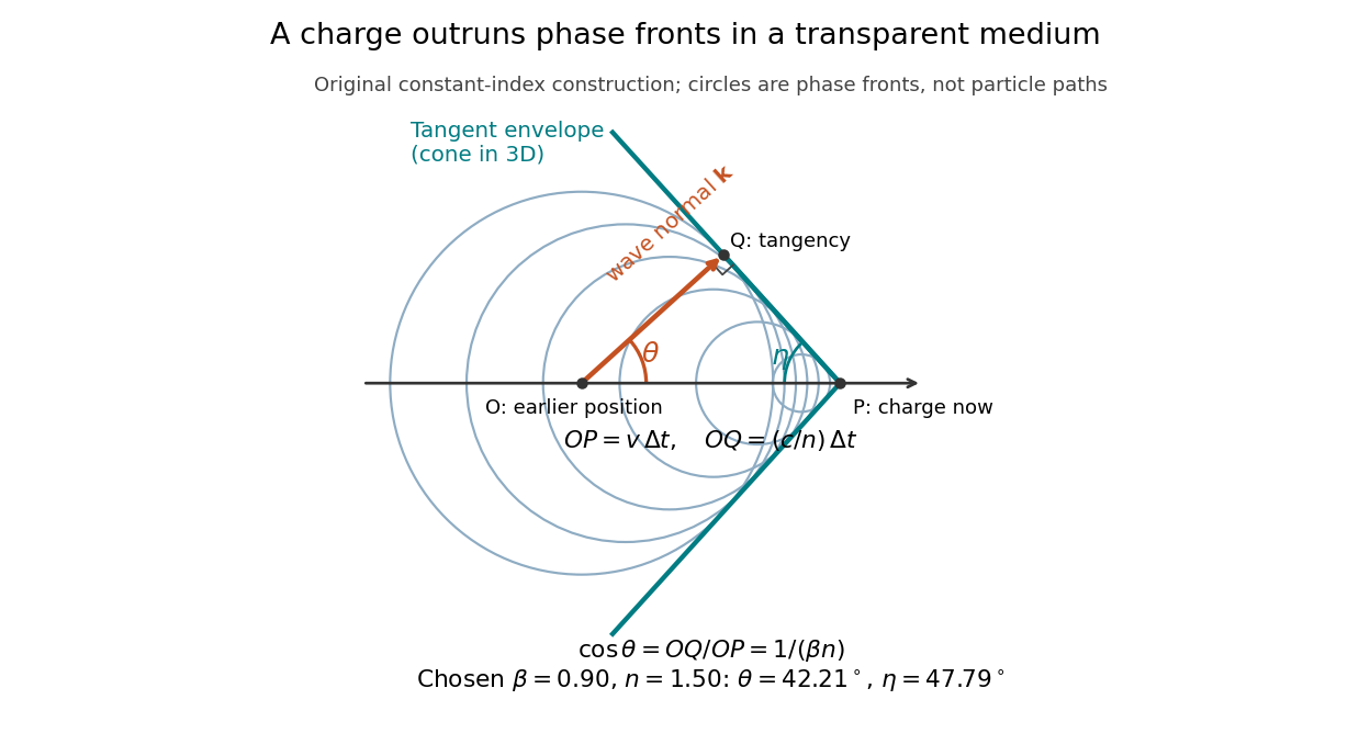
In a dispersive medium, apply the phase matching derivation separately at each angular frequency. The circle construction uses one fixed phase speed; it does not determine the envelope of a broadband wave packet. In particular, group velocity controls packet propagation under its usual narrow-band assumptions, and the simple complementary-angle construction need not describe a dispersive pulse front. A finite track also broadens the ideal directional selection: adding contributions over duration $T$ gives a factor proportional to $\sin (\Delta T/2)/\Delta$, with $\Delta =kv\cos \theta -\omega$, rather than an infinitely sharp direction.

In his 1958 lecture, Pavel Cherenkov recalls the 1934 reports by himself and Sergey Vavilov: radium gamma rays illuminated solutions and their solvents. Weak light was compared using dark-adapted human vision and threshold photometry. Heating and added fluorescence quenching agents left the solvent component and its polarization of an electromagnetic wave unchanged; parallel aqueous fluorescent controls visibly quenched. Its electric vibration direction was parallel to the exciting beam, unlike the compared polarized fluorescence. Further experiments attributed the emission to fast electrons produced by Compton scattering, rather than directly to gamma rays. These comparisons supported a mechanism distinct from ordinary luminescence.^[ref]

The evidential step is the controlled comparison, rather than the mere presence of light. A weak glow could include fluorescence from impurities; suppressing a known fluorescent control tests whether the intervention actually works. Visual threshold comparisons also require a stable observer and viewing conditions. These early controls do not themselves calibrate absolute photon yield or supply a single-electron angular scan. Its polarization of an electromagnetic wave comparison also does not by itself measure the Cherenkov cone angle of an individual electron.

Ilya Frank and Igor Tamm supplied the theory in 1937; Ilya Frank also investigated nuclear physics experimentally and later directed neutron research.^[ref] Sergey Vavilov, an optics and luminescence researcher and collaborator in the discovery, died in 1951. The 1958 Nobel Prize in Physics went to Pavel Cherenkov, Ilya Frank and Igor Tamm; Sergey Vavilov was not a recipient.^[ref]

For a charge moving at $v=\beta c$, the Cherenkov radiation photon direction makes angle ${\theta }_C$ to the trajectory with $\cos {\theta }_C=1/(n\beta )$. The full cone of photon directions has opening $2{\theta }_C$. The corresponding conical wavefront is perpendicular to those directions and has half-angle $\mu =\pi /2-{\theta }_C$, satisfying $\sin \mu =1/(n\beta )$. Therefore a full opening angle $\alpha$ gives $n=1/[\beta \cos (\alpha /2)]$ for the photon-direction cone, but $n=1/[\beta \sin (\alpha /2)]$ for the wavefront cone. These are different geometrical definitions, not competing approximations to the same angle.

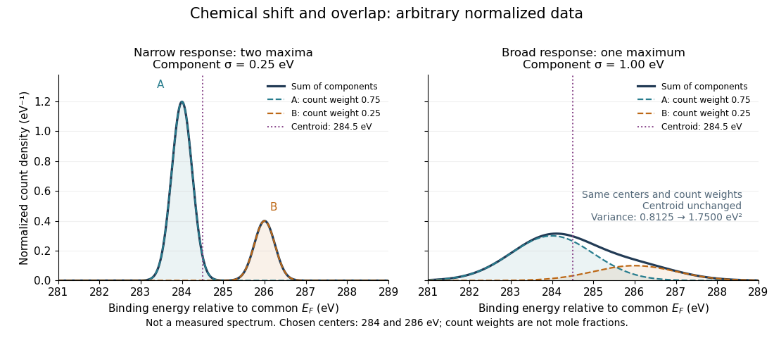
Choose two hypothetical environments A and B of one chemical element, with line centers ${\mu }_A=284\mathrm{eV}$ and ${\mu }_B=286\mathrm{eV}$. Model each line by a normalized Gaussian function with common standard deviation $\sigma$, and stipulate integrated count weights $w_A=3/4$, $w_B=1/4$. On the binding energy axis $E$, the normalized count density isAll energies in this expression use electronvolts. Each component's integrated area equals its count weight, and $\int I(E)dE=1$. There is no background, statistical counting fluctuation, or additional emission feature in this stipulated model. These choices deliberately isolate photoelectron peak overlap and resolution.

Direct integration, or the law of total expectation applied to the component label, gives the centroidThe centroid lies between the chemical environments and is not either component's binding energy. Expanding $(E-\bar{E}{)}^2$ within each component, the odd cross term integrates to zero. The resulting variance isFor $\sigma =0.25\mathrm{eV}$ the variance is $0.8125{\mathrm{eV}}^2$ and the two maxima are separated. For $\sigma =1.00\mathrm{eV}$ it is $1.7500{\mathrm{eV}}^2$ and there is one maximum. Each Gaussian's full width at half maximum is $2\sqrt{2\ln 2}\sigma$, approximately $0.589$ and $2.355\mathrm{eV}$ respectively. The chemical separation remains $2\mathrm{eV}$ in both cases. The number of visible maxima therefore does not equal the number of chemical components.

One interpretation of this change is additional independent Gaussian instrument blur. The convolution of probability densities adds the variances, so broadening $\sigma =0.25$ to $1$ requires response standard deviation $\sqrt{1-0.25^2}=\sqrt{15}/4\simeq 0.968246\mathrm{eV}$. A normalized response with zero mean preserves the centroid and integrated counts. Real line shapes and backgrounds can depart from this model, and separating hidden components is an inverse problem; a plausible fit does not alone establish uniqueness.

Finally, count weights describe detection. In a simple response model, let $n_i$ denote the number of emitting sites sampled in environment $i$, $s_i$ its effective photoionization cross section, and $T_i$ the probability that its emitted electron contributes to the selected measured line. ThenThe common factor $C$ includes exposure. Here $T_i$ includes escape from the sample, analyzer transmission and detection. Count weights equal site fractions only if the relevant response factors are equal or corrected. They are not automatically molecular mole fractions; different molecules can supply different numbers of the selected emitting sites. In an original example, equal site numbers with $s_A{T}_A=3s_B{T}_B$ give the plotted $3:1$ count ratio despite a $1:1$ site ratio.

A quasi-Fermi level is a local electron or hole population parameter in a semiconductor driven out of equilibrium, assuming each population is internally close enough to thermal equilibrium to use a Fermi-Dirac distribution. Separate electron and hole parameters replace one common equilibrium chemical potential. Their spatial profiles depend on transport, generation and recombination as well as electrostatics. For ideal ohmic contacts with the p voltage $V$ relative to n, the contact electron electrochemical potentials obey ${\mu }_p-{\mu }_n=-eV$.

The J/psi meson is the ground spin-triplet S-wave vector state of charmonium, with leading valence content $c\bar{c}$ and quantum numbers $J^{PC}=1^{--}$. It has zero net charm and can decay into hadrons or charged-lepton pairs.^[ref]

Its comparatively narrow decay width makes it a conspicuous resonance in reconstructed mass distributions. An electron–Positron mass peak in a fixed-target experiment and an enhanced event rate during an energy scan in an electron-positron collider were complementary observations in the Richter-Ting independent J/psi discovery experiments of 1974.^[ref][ref] A peak's measured width also includes detector resolution or beam-energy spread, so it must not automatically be identified with the intrinsic lifetime width.

The critical coagulation concentration is the approximate electrolyte concentration separating slow, barrier-limited aggregation from rapid aggregation of a charge-stabilized colloid. In the simplest DLVO theory, increasing salt shortens the Debye–Hückel screening length and lowers the repulsive barrier until rapid aggregation is possible. It depends on particle charge, solvent, temperature and particularly counterion valence. It is a kinetic crossover, not a universal salt concentration or necessarily an equilibrium phase boundary. Aggregation just below this crossover can be reaction limited; exactly at or above the rapid-aggregation threshold, proximity to the threshold alone does not imply a small sticking probability.

A sensitive charge neutrality test lets nominally neutral gas escape from an electrically isolated vessel connected to an electrometer. A net charge per escaping molecule would leave a measurable opposite charge on the vessel. Removing stray ions and charged particles is essential. Hydrogen and helium measurements constrain charge imbalance despite different particle binding and internal motions, providing evidence for velocity-independent additive charge rather than a charge proportional to relativistic particle energy. The 1960 experiment used this efflux principle. ^[ref]

For a neutral pion pair in a state of definite relative orbital angular momentum $L$, charge conjugation interchanges ${\pi }^{+}$ and ${\pi }^{-}$. Relabelling the particle slots reverses the relative momentum and contributes $(-1{)}^L$. The individual charged-pion phase conventions cancel in the pair. Thus a neutral vector rho meson decaying strongly to a pion pair has $L=1$ and $C=-1$. A charged rho meson is taken to the state of opposite electric charge, so it is not itself a charge-conjugation eigenstate.

If $m\ge 1$ is an integer and $\mathbb{E}[|X{|}^m]<\infty$, the characteristic function has continuous derivatives through order $m$, withThus finite absolute moments justify recovering moments from derivatives.^[ref]

For a short justification of differentiation under the integral sign, the difference quotient for the $(k-1)$st derivative has integrand $(iX{)}^{k-1}{e}^{itX}(e^{ihX}-1)/h$. Its absolute value is at most $|X{|}^k$, since $|e^{iu}-1|\le |u|$ for real $u$. Lower absolute moments are finite because $|X{|}^k\le 1+|X{|}^m$. Apply the dominated convergence theorem successively, then use the same integrable bound to obtain continuity of each derivative.

For the Bernoulli distribution with parameter $1/3$, direct differentiation gives ${\phi }_B^{\prime }(0)=i/3$ and ${\phi }_B^{\prime \prime }(0)=-1/3$, agreeing with $\mathbb{E}[B]=\mathbb{E}[B^2]=1/3$. Its variance is therefore $1/3-(1/3{)}^2=2/9$. Existence and continuity of a characteristic function alone do not authorize these moment calculations: the standard Cauchy distribution, whose expected value is undefined, still has a characteristic function. The stated finite absolute moment hypothesis is a sufficient condition for the derivative formula, not an assumption built into the definition of a characteristic function.

An orthogonal change of coordinates relates two orthonormal bases of a real inner product space. With the new basis vectors as columns of an orthogonal matrix $Q$, old and new coordinate columns obey $x=Qy$. Then $x^{T}x=y^{T}y$, so Euclidean norm, Euclidean distance and angles are preserved. A quadratic form $x^{T}Ax$ becomes $y^T(Q^{T}AQ)y$. For a symmetric matrix, orthogonal diagonalization chooses $Q$ so that the transformed quadratic form is a sum of eigenvalues times squared coordinates. This explains the principal-axis descriptions of a quadric surface.

For a nondegenerate $d$-dimensional simplex $S$ with vertices $v_0,\dots ,v_d$ and an affine function $f$, the integral equals the volume times the value at the centroid $c=(v_0+\cdots +v_d)/(d+1)$. To prove this, write $x={\sum }_i{\lambda }_i(x)v_i$ in a barycentric coordinate system. On the standard simplex, symmetry permuting the vertices gives equal integrals of all ${\lambda }_i$; since ${\sum }_i{\lambda }_i=1$, each is $\mathrm{vol}(S)/(d+1)$. An invertible affine map transfers this result to any simplex. Affineness gives $f(x)={\sum }_i{\lambda }_i(x)f(v_i)$, so linearity of integration proves the formula. For a tetrahedron the factor is one quarter. The rule is exact for affine integrands; a nonlinear integrand generally needs additional moments.

Consider two equal balls of mass $m$, four light rods each of length $L$, a fixed upper pivot and a light sliding lower collar. Each upper and lower rod makes angle $\theta$ with the spindle. A spring of spring constant $k$ is uncompressed at $\theta =0$ and is compressed by collar motion. Its compression is $\delta =2L(1-\cos \theta )$. Collar balance gives $2T_l\cos \theta =k\delta$, while vertical ball balance gives $(T_u-T_l)\cos \theta =mg$. Radial Newton's second law gives $(T_u+T_l)\sin \theta =m{\omega }^{2}L\sin \theta$. Eliminating the rod tensions proves the displayed relation for nonzero $\theta$.

For total ball mass $m$, arm length $l$ and imposed constant shaft speed $\Omega$, the reduced effective potential is $V_{\mathrm{eff}}/(m{l}^2)=-{\Omega }^2{\sin }^2\theta /2-{\omega }_0^2\cos \theta$. Its equilibrium equation is $\sin \theta ({\omega }_0^2-{\Omega }^2\cos \theta )=0$. The downward state is stable for $|\Omega |<{\omega }_0$ and loses linear stability above it; nonzero stable openings then satisfy the displayed relation. Extending the angle to signed values gives a supercritical pitchfork bifurcation. Squared angular frequencies of small oscillations are ${\omega }_0^2-{\Omega }^2$ at the downward state and ${\Omega }^2-{\omega }_0^4/{\Omega }^2$ at the open states. At threshold the quadratic term vanishes but the quartic potential is positive, so zero linear frequency does not imply finite-amplitude free motion.

For $a>b>0$ with $a,b\ne 1$, the solution of $(D_t+a)(D_t+b)y=e^{-|t|}$ that decays at both infinities isIts Fourier transform is $2/[(1+k^2)(a+ik)(b+ik)]$. The lower half-plane contains only the pole $-i$, while the upper half-plane contains $i,ia,ib$. Inverting by the residue theorem gives the two expressions. Direct substitution verifies the equation separately on each side, and $y,y^{\prime }$ match at zero, so there is no spurious impulsive source. The negative-time response is nonzero because the forcing already acts before zero, even though the Green function is causal. Coinciding rates $a=1$ or $b=1$ require limits with polynomial times exponential terms.

For $x^{\prime \prime }+2\gamma x^{\prime }+({\gamma }^2+{\mu }^2)x=g(t)$ with $\gamma ,\mu >0$, zero initial data give $x(t)={\mu }^{-1}{\int }_0^t{e}^{-\gamma (t-s)}\sin (\mu (t-s))g(s)ds$. If $|g(s)|\le C{e}^{-as}$ for $a>0$, the causal Green function of a damped oscillator givesBoth bounds tend to zero. A decaying homogeneous transient can be added for arbitrary finite initial data. The coincident decay rates require the extra polynomial factor and cannot be handled by dividing by zero in the first expression.

For $\beta >0$, $0<\gamma <{\omega }_0$ and zero prehistory, the equation $y^{\prime \prime }+2\gamma y^{\prime }+{\omega }_0^{2}y=F{e}^{-\beta t}H(t)$ hasOne obtains it by convolution with the causal Green function of a damped oscillator. Alternatively, a particular exponential has amplitude $F/[(\beta -\gamma {)}^2+{\Omega }^2]$; the two homogeneous terms enforce $y(0)=y^{\prime }(0)=0$. These continuity conditions avoid adding impulsive forcing at switch-on. The forcing may have either sign; its Fourier transform is $-iF/(\omega -i\beta )$ with the negative-exponential transform convention.

With inverse Fourier transform $G(t)=\int G(\omega )e^{-i\omega t}d\omega /(2\pi )$, a tempered retarded response vanishes for $t<0$ and is analytic in the upper frequency half-plane with suitable large-frequency growth bounds. Poles strictly below the real axis describe decaying modes; upper-half-plane poles obstruct a bounded retarded real-axis Fourier response. However causality alone does not imply stability: a retarded exponentially growing Green function can exist without an ordinary Fourier transform. Its Laplace transform inversion contour must pass above the growth poles in the frequency plane. Moving the contour to the real axis changes the boundary condition and can introduce a pre-response.