
Sparse page table allocation 2026-10-14
Use the two-level address translation model and map exactly four resident virtual memory pages, numbered
0x12, 0x13, 0xa0, and 0xa1. Assign their data page frames to 0x07, 0x02, 0x05, and 0x06, respectively. Only two root indices occur: 1 and 10. Allocate exactly three table nodes: the root at 0x8000, the lower-level table for root index 1 at 0x9000, and the lower-level table for root index 10 at 0xa000. Root entries 1 and 10 reference those tables; all other root entries are absent. Lower-level entries 2 and 3 in the first table and entries 0 and 1 in the second table hold the four mappings; every other lower-level entry is absent. Use the read-only permissions already specified for virtual memory page 0x12; let the other three mappings permit user reads and writes, with no execution, and let both populated root entries permit user reads and writes.Each root index covers 16 virtual memory pages, hence bytes of the address space. A compact table node occupies bytes. The three nodes therefore require bytes of table storage, including the root and all absent entry slots in the allocated nodes. A single-level array requires bytes for the same address space, saving bytes in the compact model. Four data page frames occupy another bytes; those contents are separate from table storage.
If instead the allocator dedicates a whole 256-byte page frame to every table node, the three nodes consume 768 bytes, leaving bytes unused within those allocations. The single-level table fills four such page frames and still consumes 1024 bytes. Thus this example saves 256 bytes of allocated table storage under that alternative policy. Neither accounting includes allocator metadata, operating-system process records, or translation lookaside buffer storage; data allocations are the same in both designs.
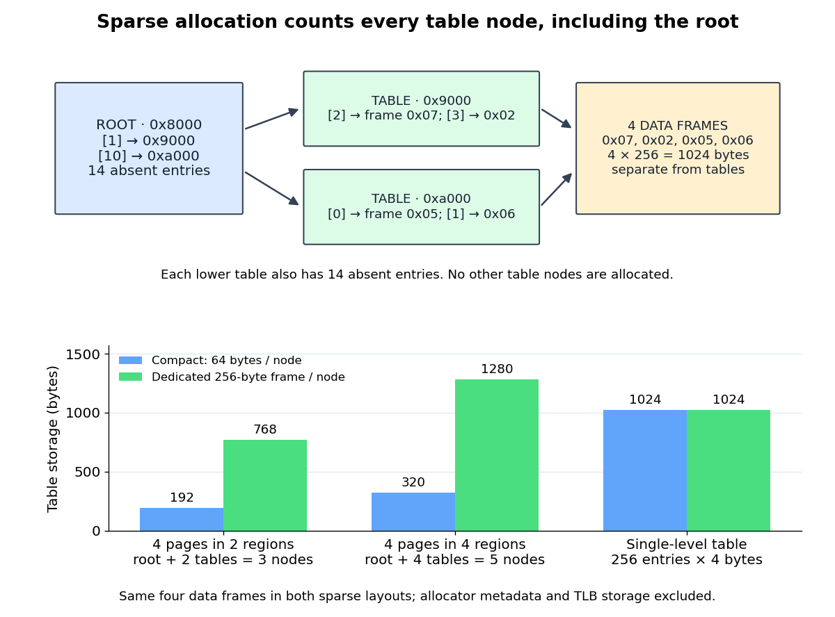
All table nodes for four mapped pages, and the footprint change when the same four pages occupy four root regions
. Details. Placement matters as well as mapping count. Four virtual memory pages
0x12, 0x42, 0x72, and 0xa2 require the root plus four lower-level tables: five nodes, 320 compact bytes, or 1280 bytes with a dedicated page frame per node. Only four data page frames are still required. Let be the number of distinct root indices represented by the mappings. With no retained empty lower-level tables, table storage is compact bytes or allocated bytes under the dedicated-page frame policy. Even an empty address space retains the root in this accounting, so costs 64 or 256 bytes.For a fully populated address space, : 17 nodes cost 1088 compact bytes or 4352 allocated bytes. The single-level table remains 1024 bytes. Sparse allocation is therefore a conditional space benefit; scattered mappings, node allocation granularity, and the root's overhead can reverse it. Additional dependent lookups on a TLB miss also have a cost, but node counts alone establish no universal execution-time ordering.
Two-level address translation 2026-10-14
Choose an original teaching model with 16-bit virtual addresses, 16-bit physical addresses, and 256-byte memory pages and page frames. The eight high bits identify a virtual memory page; divide these into two four-bit indices. The eight low bits are the offset within the memory page. Thus each page table has 16 entries: the root selects a lower-level page table, and that table selects a data page frame. Every page table entry is four bytes, including its reference and flags. These are chosen model parameters, not a hardware entry encoding.
For a virtual address , extract the root index , lower-level index , and offset by Euclidean division:Here is the floor function and denotes the remainder in Euclidean division. Each index ranges from 0 to 15, and ranges from 0 to 255. In hexadecimal, virtual address
0x1234 splits into , , and ; its binary numeral system representation is 0001 | 0010 | 00110100.Fix the requested operation to be a one-byte user read. Assume both table nodes and the data page frame are resident, table reads are allowed, and no mapping changes during the page table walk. The model requires presence at both levels and takes the set intersection of the two entries' read, write, execute, and user-access permissions. This is an explicit memory protection rule for this model; Sv39 page tables use different rules. The root's physical address is
0x8000; the relevant entries are:| Record | Physical address of record | Reference held in the page table entry | Presence and permissions |
|---|---|---|---|
| Root entry 1 | 0x8000 + 1*4 = 0x8004 | Lower-level table at 0x9000 | Present; user; read/write; no execute |
| Lower-level entry 2 | 0x9000 + 2*4 = 0x9008 | Data page frame 0x07, base 0x0700 | Present; user; read-only; no execute |
The first lookup obtains a table reference, not the final data physical address. The second lookup obtains page frame number 7. Both entries permit a user read, so the original offset is added to the data page frame base:The page table walk therefore reads records at
0x8004 and 0x9008, then the requested read accesses data at 0x0734. All three are distinct physical addresses. These are two dependent table lookups followed by one data access, not a claim of three accesses to main computer memory: a memory cache can satisfy table lookups, and cached intermediate translations can skip them.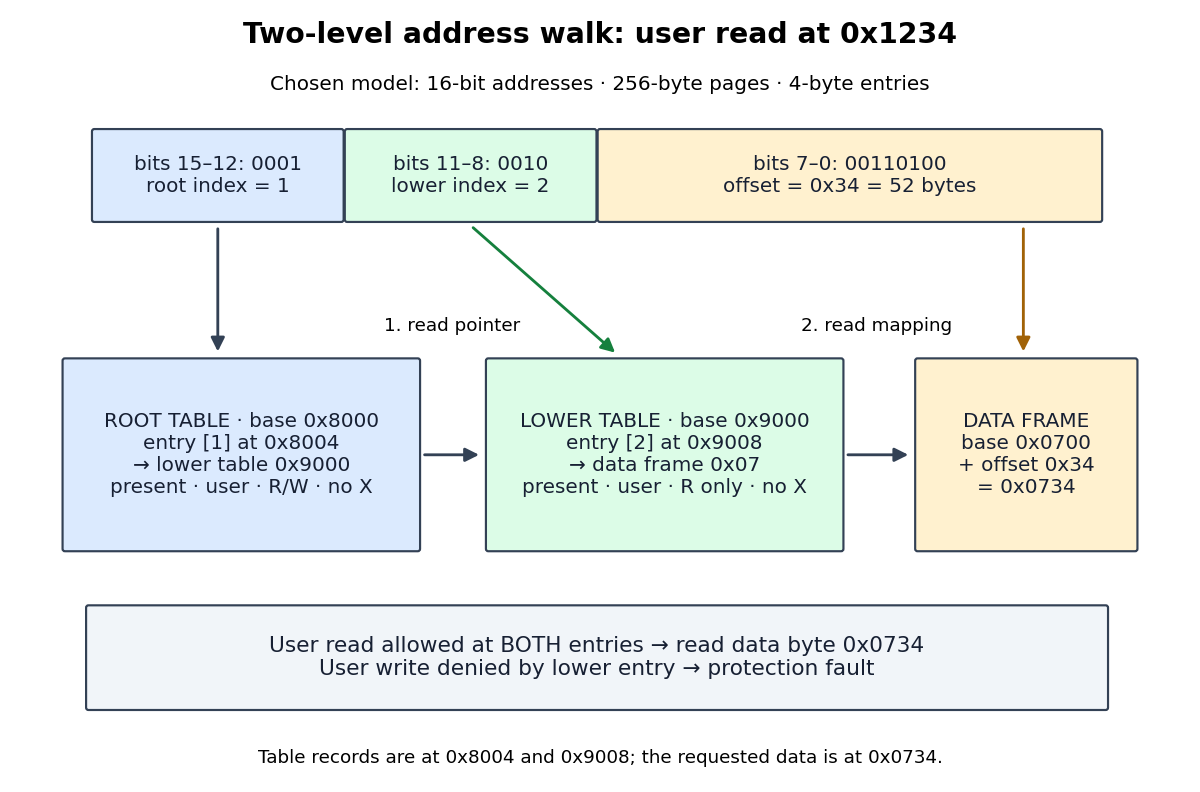
Under the same memory protection rule, a user write at
0x1234 fails because lower-level entry 2 denies writes, even though root entry 1 allows them. Clearing either entry's presence flag also prevents the access. An absent root entry stops the page table walk before any lower-level lookup. A page fault then requires the operating system to determine whether a permitted mapping needs storage or the access is invalid; absence alone does not establish demand paging eligibility.With an empty translation lookaside buffer, the permitted read causes a TLB miss and this successful page table walk, with no page fault. If the resulting mapping and permissions are cached for the current address space, a later read at
0x1235 can use a TLB hit to reach 0x0735. A later write can cause a protection page fault on a TLB hit because the cached mapping remains read-only. Assume cached permissions are current; changing them requires the architecture's prescribed invalidation. A TLB miss describes a missing cached translation, while a page fault describes an access that cannot proceed under the translation or protection rules. [ref]Page Tables by The kernel development community. MMU, TLB, and Page Faults: translation caches, page walks, and faults for missing or forbidden mappings
Moving-average polynomial 2026-10-14
The moving-average polynomial records the coefficients of the finite noise filter. Evaluating it at the backshift operator gives . In a reduced ARMA representation, invertibility is equivalent to having no roots in the closed unit disc.
Multivariate moving-average model 2026-10-14
A multivariate moving-average model filters vector white noise through fixed matrix coefficients. If the noise has zero mean and lag-zero covariance matrix , with all nonzero-lag cross-covariances zero, then the filtered process is a weakly stationary process. With the convention , its covariance matrix is , omitting terms outside the filter range. Positive and negative lags satisfy .
At a nondegenerate critical point placed at the origin, integral Taylor theorem gives , where is a smooth symmetric matrix and . A constant linear change makes diagonal with entries . Successive completion of squares, with the Schur complement at each step, produces a smooth invertible triangular matrix such that . The pivots keep their nonzero signs near zero. The map has invertible derivative at zero, so the inverse function theorem makes it a coordinate system. The signs are the Hessian matrix signature by Sylvester's law of inertia.
Morse inequalities 2026-10-14
For a closed manifold and a Morse function, the displayed strong inequalities hold for every , with equality at the top dimension. Indeed the Morse chain complex rank formula makes the alternating sum equal to . Adding the inequalities at and gives . The weak inequalities, even together with equality of Euler characteristics, are less restrictive: and satisfy those numerical conditions but violate the strong inequality at .
Morse-Smale complex 2026-10-14
Here is the signed number of unparametrized trajectories of a Morse-Smale gradient flow from to . Compactifying one-dimensional trajectory moduli spaces gives . The generators coincide with the cells furnished by the unstable manifolds, and the trajectory count is their cellular incidence number, so the complex computes integral homology.
Degree of a morphism of curves 2026-10-14
A nonconstant morphism of algebraic varieties between smooth projective integral curves is finite, and its degree is the degree of the induced extension of function fields. It is also the degree of the pullback of a rational point, with ramification multiplicities and residue degrees included: locally the finite coordinate algebra is a torsion-free module over the target discrete valuation ring, hence free of its generic rank. For and a rational function defining , the pullback of infinity is its pole divisor, so the total pole degree equals . A degree-one finite map to a normal curve is an isomorphism, since a finite integral algebra inside its unchanged function field equals the integrally closed target ring.
A -algebra isomorphism between the local rings at closed points extends to a morphism on some neighborhoods: represent the images of finitely many affine coordinate generators by fractions, and shrink where their denominators are nonzero and their finitely many relations hold. Extend its inverse the same way. The two compositions agree with the identity as germs; finitely many coordinate equalities make them identities after shrinking again. Taking inverse images of these neighborhoods then gives mutually inverse actual neighborhood isomorphisms, not just a formal-completion isomorphism.
Generically finite morphism 2026-10-14
A dominant morphism of varieties is generically finite when its extension of function fields is finite. Its degree is the degree of this field extension. A dominant morphism between integral varieties of equal dimension is generically finite; over a suitable nonempty open subset of the target its fibers are finite.
Conic bundle 2026-10-14
A flat proper morphism of algebraic varieties whose geometric fibres are plane conics, usually presented as a quadratic equation in a projective bundle of relative dimension two. The generic fibre is normally required to be smooth; singular conics can occur in special fibres. A conic bundle from a line on a smooth cubic surface has five reducible fibres over the projective line.
Morphism of algebraic curves 2026-10-14
A morphism of algebraic varieties whose source and target are algebraic curves. A nonconstant morphism between smooth projective curves is finite and surjective; its degree is the degree of the induced extension of function fields.
For a nonzero matrix , the operator norm induced by the Euclidean norm satisfies , where is its smallest positive singular value. The singular value decomposition makes the danger visible: a small nonzero stretch becomes a large amplification of errors when inverted.
For instance, when ,A data perturbation changes the reconstructed input by . At , however, the pseudoinverse is : exactly zero and merely small are different cases. Thus the pseudoinverse need not be continuous across a change of matrix rank. With uncertain data, truncated singular value decomposition or Tikhonov regularization can trade exact inversion of weak directions for stability; the cutoff or penalty adds a modelling choice.
Underdetermined minimum-norm example 2026-10-14
Now take one equation for two unknowns:The linear system has an entire affine line of exact solutions. Since has full row rank, its Moore-Penrose inverse isThe kernel is , and all exact solutions areBecause is orthogonal to ,The Euclidean norm is therefore smallest exactly at . The zero residual alone cannot select a solution; the minimum-norm rule supplies the additional criterion.
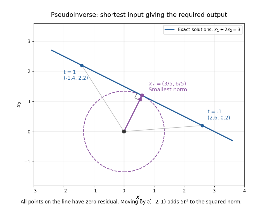
The minimum-norm solution is the closest point of the solution line to the origin
. The affine line is perpendicular to . Moving along the line changes only a kernel component and increases by . Details.This selection depends on the specified inner product. Rescaling one unknown changes what counts as a small Euclidean norm, so units and weighting matter in an application. A minimum-norm answer is mathematically canonical for the chosen geometry, rather than an automatic guarantee of physical plausibility.
Overdetermined least-squares example 2026-10-14
Suppose three measurements constrain two unknowns:The linear system asks for , , and , which are incompatible. A least-squares solution makes a balanced compromise. The matrix has full column rank, soThe fitted output and residual areThus the two direct measurements are each overshot by one, and the measured sum is undershot by one. The residual has Euclidean norm and is orthogonal to the column space, the plane in output coordinates .
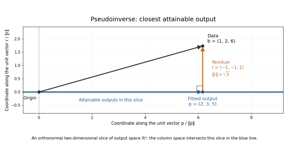
For any perturbation , the orthogonality of to givesSince the kernel of is trivial, every nonzero increases the residual. The least-squares solution is unique in this example. The formula using is convenient for these small exact calculations; an actual numerical computation can use a QR decomposition or singular value decomposition to avoid the extra conditioning cost of the least-squares normal equations. For full column rank, the squared singular values of are the eigenvalues of , so its condition number in the Euclidean norm is . [ref]
https://ocw.mit.edu/courses/18-065-matrix-methods-in-data-analysis-signal-processing-and-machine-learning-spring-2018/resources/lecture-9-four-ways-to-solve-least-squares-problems/. Strang, MIT 18.065 Lecture 9: four ways to solve least-squares problems
Libration 2026-10-14
Libration is the apparent rocking of a body as seen by an observer. For the Moon, longitudinal libration arises because orbital eccentricity makes its orbital angular speed vary while its spin is much more uniform: the direction to Earth advances ahead of, then falls behind, the mean facing direction. The Moon's tilted geometry also causes latitudinal libration; small actual rotational oscillations provide further corrections. Thus lunar synchronous rotation holds in the mean, rather than requiring exact instantaneous alignment. [ref]. [ref].
Lunar eclipse 2026-10-14
A lunar eclipse occurs when Earth blocks some or all of the direct sunlight reaching the Moon. It requires alignment near full Moon; the orbital inclination usually carries the Moon clear of Earth's shadow. Ordinary lunar phases instead arise from viewing different amounts of the sunlit hemisphere. [ref].
Lunar phase 2026-10-14
A lunar phase is the appearance of the sunlit portion of the Moon as seen from Earth. Outside a lunar eclipse, the distant Sun illuminates approximately one hemisphere of the Moon, but an observer sees a changing overlap of that hemisphere with the hemisphere facing Earth. The lunar phase therefore changes even though synchronous rotation keeps approximately the same near side of the Moon facing Earth. [ref].
The cycle runs through new Moon, waxing crescent, first quarter, waxing gibbous, full Moon, waning gibbous, last quarter and waning crescent. “Waxing” means that the lunar illuminated fraction is increasing; “waning” means it is decreasing. A crescent has less than half its apparent disk sunlit, and a gibbous lunar phase has more than half. First and last quarter each show half a disk: “quarter” refers to progress around the cycle, rather than a quarter of the disk being lit. [ref]
https://aa.usno.navy.mil/data/MoonFraction. US Naval Observatory: disk fractions and waxing versus waning
.An instructive circular orbit model puts Earth at the origin, the Sun far away along , and the Moon at . The sunward position , , gives new Moon; the opposite position , , gives full Moon. Counterclockwise motion gives first quarter at and last quarter at . The Sun's direction is fixed during this snapshot of the cycle. Every small globe in the orbital view is illuminated on its half; the adjacent apparent disks are separate views from Earth, rather than globes viewed from above.
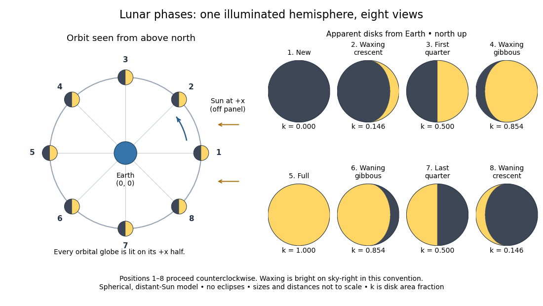
The disk views choose north up, with the upward direction perpendicular to the orbital plane. In this convention waxing lunar phases are bright on the right and waning lunar phases on the left. Local horizon orientation and viewing from different locations on Earth can rotate the apparent disk; its lit edge always points toward the projected direction of the Sun. The lunar illuminated fraction is unaffected by this rotation.
The useful angle is the phase angle , with the Sun, the Moon and the observer at Earth's center: its vertex is at the Moon. Full Moon has , quarter has , and new Moon has in the ideal model. By contrast, the elongation has its vertex at Earth. For a distant Sun, its rays are parallel, soHere is the lunar illuminated fraction: a fraction of projected disk area, not a fraction of the Moon's total surface area or its received radiant flux relative to full Moon. The phase angle and unsigned elongation each lie between and , so either alone gives the illuminated amount without distinguishing waxing from waning. The orbital direction resolves that ambiguity.
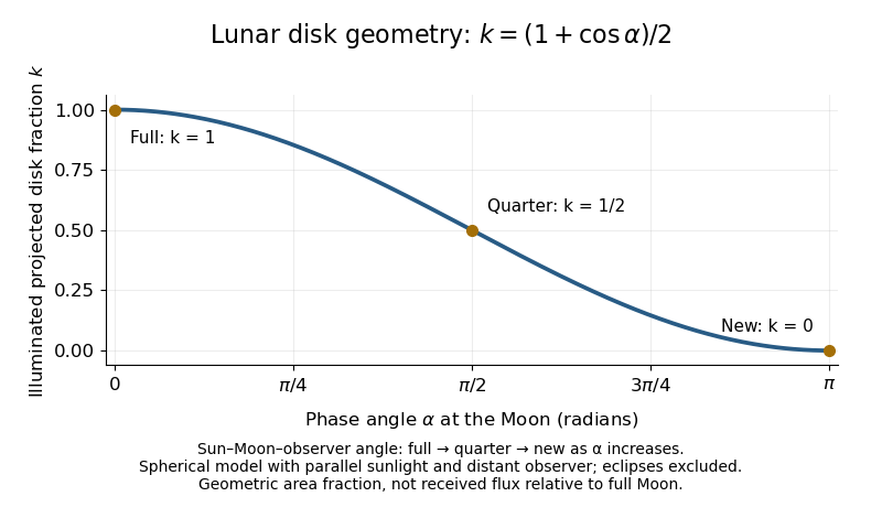


The lunar illuminated fraction has an elegant geometric derivation. Model the Moon as a sphere of unit radius and view it along the direction. Take the Sun's unit direction to be . A visible surface point above apparent disk coordinates has . Direct illumination requires the outward normal's dot product with the sunward direction to be positive. The day-night terminator therefore obeys . At a fixed , set ; the visible day-night terminator is , and the illuminated strip extends from to the right edge . Integrating its width givesThe integral is the area of half a unit circle. Thus a three-dimensional visibility problem reduces to a circle's area and a cosine. The derivation assumes parallel sunlight, a distant observer and a sphere, and ignores a lunar eclipse. Real observed brightness additionally depends on surface scattering of light and observing geometry, so does not promise half the full-Moon radiant flux.
For a worked example, elongation gives phase angle and : a crescent with of its apparent disk sunlit. At elongation , the phase angle is and : a gibbous lunar phase. At , . In each case the same occurs once while waxing and once while waning in the ideal cycle.
Ordinary lunar phases are not caused by Earth's shadow. A lunar eclipse occurs only when the Moon actually enters that shadow near full Moon. The orbital inclination of the Moon is about relative to Earth's orbital plane around the Sun; most full Moons pass above or below the shadow. This is why full Moon does not imply a lunar eclipse every month. [ref]
https://science.nasa.gov/moon/eclipses/. NASA: lunar eclipses and the Moon's roughly five-degree orbital tilt
.The phase cycle is a synodic month, about days, whereas the Moon's orbital period relative to distant stars is a sidereal month, about days. During one sidereal month, Earth advances around the Sun, so the Moon must move farther to repeat the sunward alignment. For coplanar circular orbits traversed in the same direction, subtract their mean motions: , with . HenceUsing and gives , consistent with the mean synodic month of days. After one sidereal month, the sunward direction has advanced about ; catching up takes about more days. These are mean-period estimates: orbital eccentricity and changing geometry make individual synodic months vary. [ref]
https://eclipse.gsfc.nasa.gov/SEhelp/moonorbit.html. Fred Espenak, NASA: sidereal and synodic months and varying lunations
. [ref]https://nssdc.gsfc.nasa.gov/planetary/factsheet/earthfact.html. David R. Williams, NASA: Earth's sidereal orbital period
.The lunar phase is also a practical clock for observing. Full Moon is opposite the Sun and rises roughly at sunset; first quarter is about a right angle from the Sun and is convenient in the evening, while last quarter is convenient before dawn. These are rough guides, not exact rise-time predictions for every place and season. [ref]. Historically, repeated lunar phases provided the month in lunar calendars, while half-lit disks gave Aristarchus of Samos a way to infer astronomical distances. [ref]
https://eclipse.gsfc.nasa.gov/SEhelp/moonorbit.html. Fred Espenak, NASA: lunations and lunar calendars
. Far side of the Moon 2026-10-14
The far side of the Moon is the hemisphere directed approximately away from Earth. “Far” describes the direction to Earth; it does not describe illumination by the Sun. The far side of the Moon experiences both sunlight and darkness during the lunar phase cycle. [ref].
Near side of the Moon Created 2026-10-14 Updated 2026-10-25
The near side of the Moon is the hemisphere directed approximately toward Earth. Libration changes the exact visible boundary, so synchronous rotation does not mean that an observer always sees precisely the same hemisphere.
There are unlisted articles, also show them or only show them.