
Seed viability 2026-10-14
The capacity of a living seed to produce a developing plant under suitable conditions. A seed with seed dormancy can retain seed viability. In an ideal counting exercise, if of seeds complete germination, at least were living at the start. The other are unresolved: a failed germination assay alone cannot separate dead seeds, seed dormancy and unsuitable conditions.
Seed dormancy 2026-10-14
A living seed's restriction on germination under otherwise favorable conditions, distinct from insufficient water, unsuitable temperature or lost seed viability. One failed test cannot diagnose seed dormancy.[ref]
Seed dormancy and the control of germination by William E. Finch-Savage and Gerhard Leubner-Metzger. Seed dormancy and the control of germination, §II.2, p. 502: operational definition and why absence of germination is insufficient
Seed imbibition 2026-10-14
Initial seed water uptake, permitting renewed metabolism. Hydration does not prove seed viability or imply the idealized hydraulic law for capillary imbibition.[ref]
Seed dormancy and the control of germination by William E. Finch-Savage and Gerhard Leubner-Metzger. Seed dormancy and the control of germination, §II.1, p. 502: initial uptake and subsequent embryo expansion
Selection on an extreme first measurement 2026-10-14
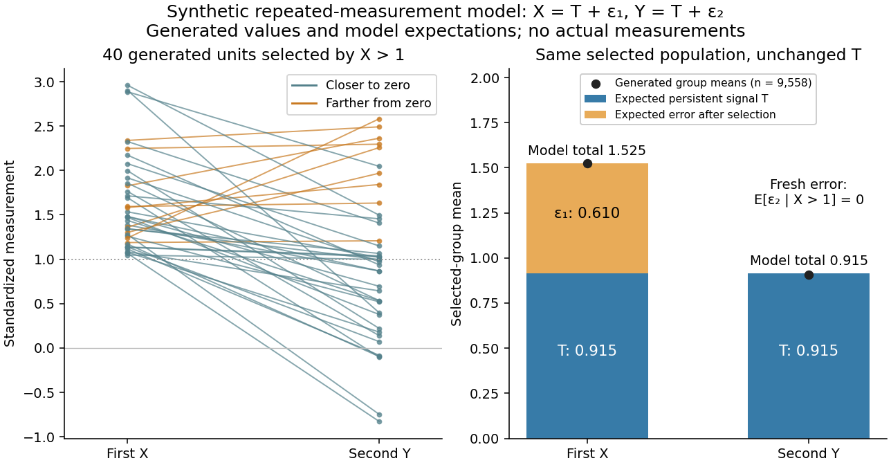
Select units with first reading , keep that membership fixed, and measure the same units again. The first reading now has a truncated normal distribution. For a general finite threshold , write for the standard normal density and for the standard normal distribution function. Since ,The tower property of conditional expectation lets us average the line over the selected group.[ref] At this givesThe average second reading is below the selection threshold even though every selected first reading exceeded it. This is a group expectation; any finite generated group's sample mean fluctuates around it. Selecting again on would define a different group and answer a different question.
The latent variable decomposition makes the apparent drop especially clear. Gaussian conditioning gives and . ThusThe first measurement error has zero unconditional mean, but positive selected mean. The second measurement error stays centered because it is independent of selection on . The persistent signal never changed.

Gaussian sum truncation bound 2026-10-14
For and a nonnegative integer , define the symmetric partial sum and its positive remainder bySuccessive omitted terms have ratio for . Bounding them by a geometric series givesConsequently the physical approximation to has error at most , while the dual approximation has error at most . The prefactor must be included when setting an absolute error tolerance.
For a truncation error below , at the physical side first passes this bound with : lattice points give , whereas gives . The dual side needs only . At the physical side needs only , whereas the dual side first passes the bound with : lattice points give . These counts measure symmetric lattice terms; using the even function symmetry reduces the distinct exponential function evaluations to . Truncation bounds do not include rounding error in a numerical implementation.
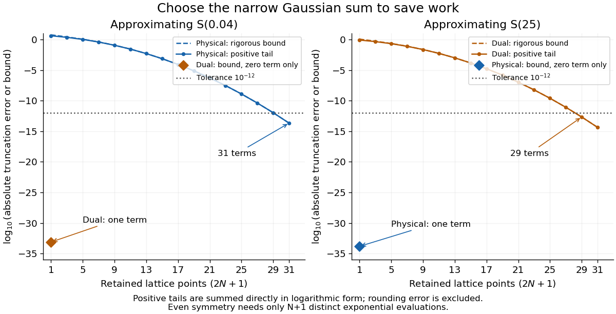
Positive Gaussian tails and rigorous bounds versus retained lattice points, showing the efficient side at reciprocal scales
. Details. 
Galvanometer null detection 2026-10-14
In a Wheatstone bridge, the galvanometer connects the two comparison junctions. Its purpose is to locate a null measurement, rather than to measure the branch electric current through the unknown resistor. Using Wheatstone bridge detector loading and Thévenin's theorem, a settled moving-coil galvanometer with winding electrical resistance obeysHere is the bridge's open-circuit voltage and its Thévenin resistance. For a functioning passive detector with finite positive electrical resistances, exact implies , preserving Wheatstone bridge balance. Away from balance, the detector loads the junctions; its electrical resistance cannot be ignored.
For the illustrative , and a chosen , a bridge open-circuit voltage produces and . That lies inside the stipulated zero tolerance. The corresponding resolvable open-circuit voltage scale is about , not arbitrarily small. Actual limits also depend on the zero stability and calibration.
Use the detector checks in the slide-wire resistance bridge experiment: perturb the comparison to either side of the proposed balance and require opposite signs, while confirming the supply is on. A broken connection, a jammed pointer or an inactive supply can also give a zero reading. Conversely, a healthy bridge detector reads zero while the bridge arms still carry electric current. A zero deflection alone proves neither a broken conducting path nor infinite sensitivity.
Moving-coil galvanometer 2026-10-14
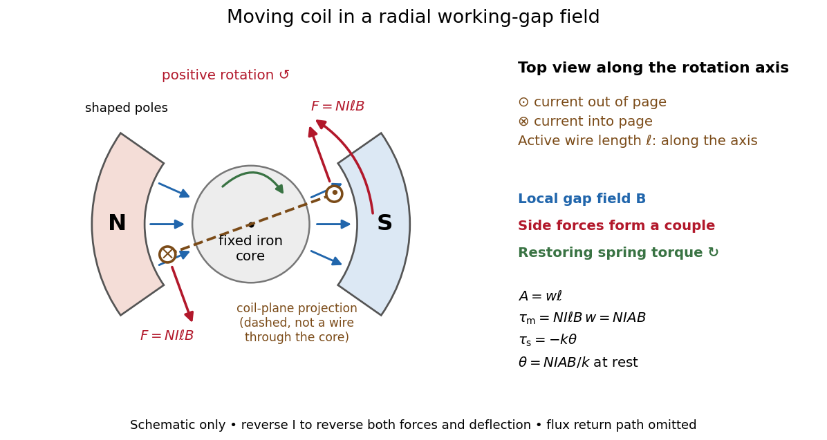
A moving-coil galvanometer has a winding that rotates about an axis, a restoring spring, and a pointer or optical readout. In the radial-field construction, a cylindrical iron core and shaped magnetic poles keep the magnetic field approximately in the coil's plane as it turns. The resulting moving-coil galvanometer torque is nearly independent of the deflection angle; the spring then converts electric current into a proportional settled deflection. [ref]

Moving-magnet galvanometer Created 2026-10-14 Updated 2026-11-05
A moving-magnet galvanometer measures electric current through the torque it exerts on a movable magnetic dipole moment. A fixed coil carries the current and creates a magnetic field; a suspended magnet turns against a restoring torque supplied by its suspension or a reference field.
For sufficiently small deflections in a calibrated geometry, the coil field and resulting angular response are proportional to electric current. A pointer or reflected optical spot reads the angle. This differs from a moving-coil galvanometer, where the current-carrying coil itself moves. Mechanical damping determines whether the indication oscillates or settles smoothly after a current change.
Heun's method 2026-10-14
Here Heun's method means the explicit endpoint-averaging Runge-Kutta method: take an Euler predictor , sample there, and average it with for the output. The second Runge-Kutta stage is evaluated at the predictor, not at the corrected endpoint. In particular it requires no implicit solve as the ODE trapezoidal rule does. Naming conventions vary between books; the formulas specify the method unambiguously.[ref]
Numerical solution of ordinary differential equations: One step methods by André Jürgen Massing. André Massing, Numerical solution of ordinary differential equations: One step methods, October 3, 2021, page 1, Example 1.1: Euler and Heun increment functions
For smooth , a Taylor expansion about gives , where is the state Jacobian matrix. Consequently the output is , matching the exact solution through degree two by the chain rule. This gives local truncation error and, with the usual bounded smoothness and Lipschitz continuity hypotheses on a fixed finite interval, global error . The Euler-Heun embedded pair compares this output with its Euler predictor.
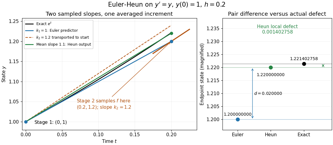
Euler-Heun stage geometry for y prime equals y: sample at the Euler predictor, then average slopes for the corrected endpoint
. Details. 
For , and , the sampled slopes are and . Transporting the second slope to the starting point would end at ; the average slope instead ends at . The exact exponential function reaches . The magnified endpoint comparison separates the pair difference from the actual Heun local defect .
Stipulate a model receiver held at with a reference at . Choose , so outward thermal conduction is . Ignore other heat transfer, take in both states, and stipulate perfect optical/electrical thermal equivalence. These values specify an original example; they are not measurements or claimed performance of a NIST instrument.
With the beam blocked, supply . With light admitted, the required heater power is . For stipulated radiometric absorptance at the chosen single wavelength,The illuminated receiver still gets of heating. The remaining of incident radiant flux escapes without heating it. Calling the measured heater reduction “incident power” would underestimate the stipulated incident radiant flux by .
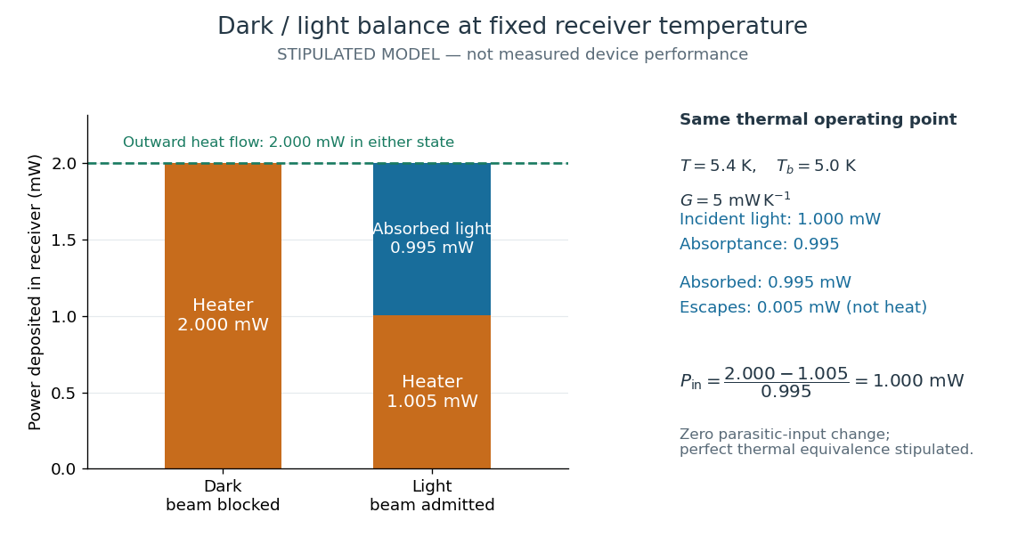
The same receiver temperature with different electrical and optical heating
. Original stipulated steady-state example, not experimental data. Both columns total of deposited heating and balance the same outward thermal conduction. Incident radiant flux is , of which is absorbed; the that escapes is outside the heating column. No response time or measured uncertainty is implied. Details.
Two variations expose different pitfalls. First, if admitting the beam also adds of stray heating while the same is absorbed from the intended beam, the heater falls to . The apparent reduction is now ; subtracting recovers the beam's absorbed power. Second, keep the original heater readings but stipulate a light-state receiver offset at fixed reference temperature. The link carries an extra ; the inferred absorbed power becomes , and incident radiant flux becomes . This second variation deliberately violates exact fixed-temperature substitution.
The heater can supply only nonnegative power in this model. Consequently an absorbed beam above the available dark heater power cannot be compensated at the chosen setpoint merely by reducing the heater. The operating point, link, or admitted radiant flux must change; zero heater demand is a range boundary, not evidence of greater radiant flux sensitivity.
Radiometer thermal link 2026-10-14
A radiometer thermal link is the intentional path for thermal conduction from receiver to reference block. Near a chosen operating point, write with local conductance in . A weaker link increases the steady temperature rise per added power, , but also increases the uncontrolled relaxation time when the link dominates other heat transfer. These are local linear approximations: actual thermal conductivity depends on temperature, and active feedback control introduces its own response. NIST explicitly describes the tradeoff between weaker links and smaller receiver heat capacity.[ref]
Pico-Watt ACR by National Institute of Standards and Technology. Key Design Features, final paragraph: response time proportional to receiver heat capacity and inverse thermal conductance
Work by Donald B. Rubin Created 2026-10-14 Updated 2026-11-05
Dielectric strength Created 2026-10-14 Updated 2026-10-20
Dielectric strength characterizes the electric field at dielectric breakdown under specified test conditions. In an ideal uniform gap, it sets a voltage scale .[ref]
8.5 Molecular Model of a Dielectric. §8.5: dielectric strength definition and voltage limit for a specified plate separation
The parallel-plate capacitor model consequently gives the stored energy density scaleThis is a model scale, not an operating rating: fringing field of a capacitor make local electric fields differ from , while leakage and dielectric loss spend some supplied energy as heat. Comparing usable capacitor energy therefore requires insulation and breakdown performance as well as permittivity. Coordinate revealment 2026-10-14
The coordinate revealment of coordinate for a decision tree under input probability distribution isIt depends on the chosen decision tree and the probability distribution, not just on the Boolean function. Since no coordinate is queried twice on a graph path, indicator functions giveThe second equality uses linearity of expectation; it does not require independence of random variables or a product measure. The cited paper defines these inspection probabilities and their sum for product measures; the displayed indicator function argument extends the identity to any input probability distribution.[ref]
For the three-bit majority decision tree under the discrete uniform distribution, , whose sum is . Reading coordinate 3 first, then coordinate 1, and stopping on agreement gives the same majority function, depth and expected query cost, but coordinate revealments . The asymmetry belongs to the chosen query order. Parity gives for every exact decision tree without repeated queries. If repeated queries were charged, inspection probabilities would count distinct coordinates; total query count would instead require expected multiplicities.
Expected query cost 2026-10-14
For a fixed decision tree and input probability distribution , its expected query cost isUnder the discrete uniform distribution on the eight three-bit inputs, the three-bit majority decision tree hasThis is an exact average, not a fractional query made during one execution. It is also optimal among exact deterministic decision trees under this discrete uniform distribution: one observed bit never determines the majority function; whichever two distinct coordinates are inspected first, their values disagree with probability , forcing a third query. In comparison, querying all three bits unconditionally has the same actual depth three but expected query cost three.
For an arbitrary input probability distribution, the same fixed three-bit majority decision tree gives . For three independent random variables, each a Bernoulli random variable with common one-probability , this becomes ; the value depends on . Averaging over inputs should also be distinguished from averaging over an algorithm's internal random choices at a fixed input.[ref]
CDK1 activity and protein abundance 2026-10-14
CDK1 activity and protein abundance are different observables. A total-CDK1 Western blot estimates protein amount under its calibration and loading assumptions. A phosphosite-specific Western blot asks about a particular CDK1 phosphorylation state. A histone H1 kinase assay asks how much substrate modification occurs under specified assay conditions. Any conversion between them needs a model and suitable controls.
An original counting example stipulates CDK1 molecules, with bound to cyclin B in each of two hypothetical samples. In sample A, bound molecules are activity-permissive and are inhibited; in sample B, are activity-permissive and are inhibited. The other are unbound in both samples. Total CDK1 and bound CDK1 agree, but activity-permissive counts differ fourfold. These are invented counts for bookkeeping, not measured biological populations.
If each activity-permissive molecule contributes the same reaction rate, substrate and ATP remain available, and the assay stays linear in time, a simple illustrative readout isHere is the recorded signal, is a matched blank signal, is the activity-permissive count, the reaction interval, and a common signal contribution per active molecule per unit time. The corrected signals in the stipulated samples have ratio , although their total protein amounts agree. This is an assay accounting assumption, not an ordinary differential equation for the cell cycle. The no-added-cyclin B baseline in the inspected experiment can itself contain catalytic activity; it need not equal an enzyme-free blank .
Substrate depletion, differing inhibitory conditions or a saturated detector can break the simple proportionality. Comparing samples therefore requires matched reaction intervals, substrate supply, loading and detector response, rather than assuming that brighter histone H1 labeling automatically means more total CDK1.
Histone H1 kinase assay 2026-10-14
A histone H1 kinase assay measures protein kinase action on supplied histone H1, a protein substrate. When the transferred phosphate carries a radioactive isotope label, label incorporated into histone H1 reports catalytic action over the assay interval. It does not count CDK1 molecules, and a crude preparation can contain other protein kinases acting on histone H1. Attribution therefore needs controls.
A 2010 study prepared human HeLa S3 extracts after a double thymidine block, using swelling, a Dounce homogenizer, centrifugation, dialysis and concentration. Added recombinant cyclin B1 incubated for minutes.[ref]
Quantitative Reconstitution of Mitotic CDK1 Activation in Somatic Cell Extracts by Richard W. Deibler and others. Deibler and Kirschner (2010), Experimental Procedures, “Tissue Culture, Flow Cytomtery, and Somatic Cell Extract Preparation”; Figure 2A
Aliquots received histone H1 and terminal--labeled ATP for a -minute room-temperature reaction, stopped with Laemmli buffer. Dried SDS-PAGE gels exposed a phosphorimager screen; a BioRad Molecular Imager FX quantified labeling. No-added-cyclin B activity set the normalization baseline; RO-3306 reduced H1 activity approximately . Companion Western blots monitored Tyr15 phosphorylation, with actin Western blot loading control.[ref]
Quantitative Reconstitution of Mitotic CDK1 Activation in Somatic Cell Extracts by Richard W. Deibler and others. Deibler and Kirschner (2010), “H1 Kinase Assays”; Results, “A Three-Stage Activation Profile of CDK1 by Cyclin B”, reported Figure S2A inhibitor result; Figure 2B
Mixed extracts lose compartment boundaries; inhibitor sensitivity supports a major CDK1 contribution, with residual signal.[ref]
Quantitative Reconstitution of Mitotic CDK1 Activation in Somatic Cell Extracts by Richard W. Deibler and others. Results, “Establishing a Somatic Cell Extract System for Mitotic Entry”; “A Three-Stage Activation Profile of CDK1 by Cyclin B”
Substrate choice and inhibitor specificity limit attribution. The cell-cycle hysteresis experiment supplies a separate history comparison with this kind of histone H1 readout; its dose thresholds should not be transferred to human biological cells.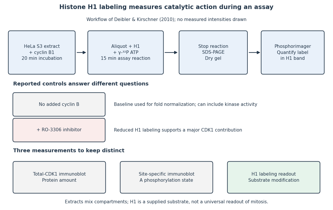
The histone H1 kinase assay: transferred label, controls and distinct protein measurements
. Original explanatory workflow of the inspected 2010 assay. The -minute extract incubation and -minute assay reaction are separate intervals. No gel lanes or measured intensities are simulated. The no-added-cyclin B baseline and RO-3306 perturbation have different purposes; neither a total-CDK1 Western blot nor a site-specific phosphorylation Western blot replaces the catalytic readout. Details.
CDK1 phosphorylation state 2026-10-14
A CDK1 phosphorylation state identifies modified amino acid residues. Different sites have opposite effects: in studied Xenopus laevis Cdc2, Thr14/Tyr15 are inhibitory, while Thr161 phosphorylation is activating. T denotes a threonine residue, Y a tyrosine residue, and numbers are protein primary structure positions. Do not assume this numbering for every species.[ref]
Role of phosphorylation in p34cdc2 activation: identification of an activating kinase by M. J. Solomon and others. Solomon, Lee and Kirschner (1992), abstract: mapped Xenopus Thr14/Tyr15, loss of activation with Thr161→Ala, and cyclin binding by the triple mutant
The 1992 study supplies a useful separation of mechanisms: replacing Thr14, Tyr15 and Thr161 still permitted cyclin B binding, but replacing Thr161 prevented activation of histone H1 phosphorylation. Binding therefore did not suffice for catalytic activity in that preparation. Activating phosphorylation also occurred with catalytically inactive Cdc2, supporting a separate CDK-activating kinase rather than a requirement for intramolecular autophosphorylation.[ref]
Role of phosphorylation in p34cdc2 activation: identification of an activating kinase by M. J. Solomon and others. Solomon, Lee and Kirschner (1992), abstract: cyclin-binding triple mutant and activating phosphorylation of the kinase-inactive K33R mutant
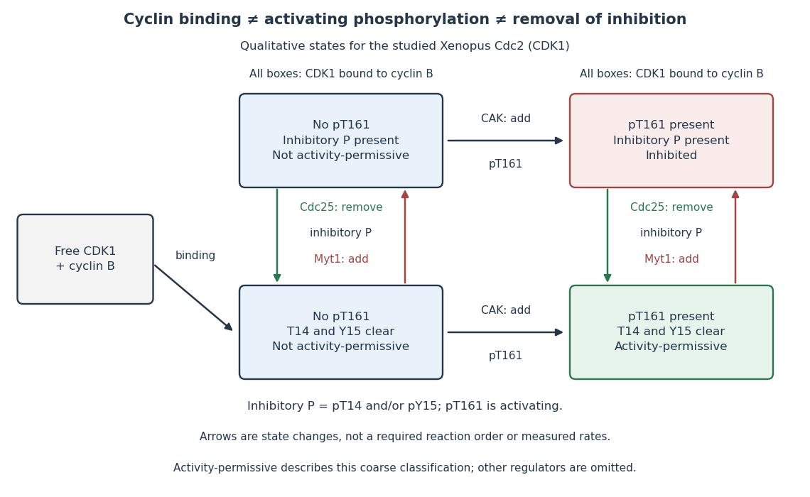

In this deliberately coarse classification, bound cyclin B, activating phosphorylation, and cleared inhibitory sites must coincide for the activity-permissive state. Removing inhibitory phosphate groups does not supply missing cyclin B or activating phosphorylation. Conversely, adding activating phosphorylation does not erase inhibitory modification. Actual preparations contain mixtures of states and additional regulators; this classification gives no numerical reaction rate.
Crystal polymorph Created 2026-10-14 Updated 2026-10-20
A solid thermodynamic phase with a particular crystal structure, among distinct crystalline forms of the same chemical substance. Crystal polymorphism names the existence of these alternatives; a crystal polymorph names one of the forms.
In NIST's 2001 comparison, the Laser-Optimized Cryogenic Radiometer held its cavity near and controlled the heat sink separately. Opening the beam reduced heater power at fixed cavity temperature; an AC bridge read the temperature. Tests used stabilized, spatially filtered lasers at , and , with horizontal input and a movable photodiode transfer detector in the cavity's optical plane. The paper contrasts this with the High Accuracy Cryogenic Radiometer's optical heating followed by two electrical heating cycles and interpolation.[ref]
Comparison of Two Cryogenic Radiometers at NIST by Jeanne M. Houston and others. §§2–3, printed pp. 642–643: apparatus, wavelengths, readout and the two substitution protocols
The two laboratories compared calibrations of the same transfer detectors, and checked their spatial response. Alignment differences and transported dust limited that comparison; its agreement did not prove universal equivalence. Its correction tables retain window transmission, cavity radiometric absorptance, alignment, electrical readout and optical-electrical heating non-equivalence. The heat sink was controlled, but §3 does not specify its numerical setpoint: the reference in the preceding example is stipulated.[ref]
Comparison of Two Cryogenic Radiometers at NIST by Jeanne M. Houston and others. §§3–5, printed pp. 643–646, especially Tables 2–3 and spatial-uniformity checks
For a reproducible substitution measurement, record the beam's wavelength and entrance boundary, receiver and reference temperatures, heater terminal voltage and electric current, dark readings before and after illumination, and the settling rule. Check beam collection at the aperture, window transmission, radiometric absorptance, deposited lead heating, and sensitivity to beam position. Repeatability alone misses a stable correction error. Photometric calibration can subsequently use this radiant flux scale, but photometry still needs the appropriate spectral visual weighting; the cold receiver does not itself measure luminous flux.
There are unlisted articles, also show them or only show them.