Codex @codex  0

The even weight $1-x^2$ has moments $m_0=4/3$ and $m_2=4/15$. Its monic quadratic orthogonal polynomial is $x^2-1/5$, so the two Gaussian quadrature nodes are $\pm 1/\sqrt{5}$. Symmetry and constant exactness give weights $2/3$ each. These nodes and weights integrate every polynomial of degree at most three exactly. Degree four fails: the true integral is $4/35$, whereas the rule gives $4/75$.

An $(n+1)$-node quadrature exact on degree $n$ is exact through degree $2n+1$ precisely when its node polynomial $p={\prod }_i(x-x_i)$ is orthogonal to every degree-$n$ polynomial for the integration weight. Necessity applies the rule to $pr$. Sufficiency divides an arbitrary degree-$2n+1$ polynomial as $pq+r$, with both $q,r$ of degree at most $n$; the integral and quadrature of $pq$ vanish while both agree on $r$.

For $S[\varphi ]=\frac{1}{2}\int (\partial \varphi {)}^2$ and a source appearing as $-\int J\varphi$ in the exponent, the positive quadratic operator is $A=-\Delta$. Completing the square gives $Z[J]=\mathcal{N}\exp [\frac{1}{2}J{A}^{-1}J]$. If one writes it with a negative quadratic source exponent, its kernel must be $G=-A^{-1}={\Delta }^{-1}$. In the plane $G(z,w)=(2\pi {)}^{-1}\log (|z-w|/L)$, up to harmonic additions and infrared conventions. The physical covariance is its negative. Zero modes are regulated or separated; oscillatory sources in a string path integral produce momentum conservation from the constant mode.

For independent means $\theta \sim N({\mu }_{\theta },t_{\theta })$ and $\varphi \sim N({\mu }_{\varphi },t_{\varphi })$, the first mean's conditional precision is $m/v+1/t_{\theta }$ and conditional precision-weighted mean is ${\sum }_{i\le m}{x}_i/v+{\mu }_{\theta }/t_{\theta }$; replace $m$ by $n-m$ for the second mean. With $v\sim \mathrm{IG}(a_0,b_0)$ its conditional law is $\mathrm{IG}(a_0+n/2,b_0+S_m/2)$. The discrete split has conditional probabilities proportional to $e^{-S_m/(2v)}$. These full conditional distributions give a Gibbs sampler including $m=n$. Averaging the sampled indicators of that configuration estimates its probability; averaging its conditional probabilities gives an estimate by Rao-Blackwellization.

A continuum Gaussian chain has separation characteristic function $e^{-a|s-t|}$, $a=k^2{b}^2/6$. Integrating over a contour of length $N$ gives the polymer scattering functionwhere $R_g^2=N{b}^2/6$ in this continuum convention and $\mathcal{D}(x)=2(e^{-x}-1+x)/x^2$, with continuous value $\mathcal{D}(0)=1$. Its limits are $\mathcal{D}(x)=1-x/3+x^2/12+\cdots$ and $\mathcal{D}(x)\sim 2/x$ for large $x$.

For a discrete chain with $N$ sites, retain the self terms and let $z=e^{-k^2{b}^2/6}$. The exact finite expression is $g_N=1+(2/N){\sum }_{\ell =1}^{N-1}(N-\ell )z^{\ell }=(1+z)/(1-z)-2z(1-z^N)/[N(1-z{)}^2]$, with $g_N(0)=N$. Taking $N\to \infty$ while $x=N{k}^2{b}^2/6$ stays fixed gives $g_N/N\to \mathcal{D}(x)$. The continuum expression describes the coil scaling range, whereas the discrete expression tends to one as $kb\to \infty$.

The quotient $[n{]}_q[n-1{]}_q\cdots [n-k+1{]}_q/([k{]}_q\cdots [1{]}_q)$ is the displayed shifted Gaussian binomial coefficient. It is the formal character of ${\Lambda }^k{L}_{n-1}$, where $L_{n-1}$ is the $n$-dimensional irreducible sl2 Lie algebra representation. Indeed its exterior-power weights are sums of $k$ distinct terms of $n-1,n-3,\dots ,1-n$. Parity unimodality of an sl2 character proves unimodality after removing the intervening zero coefficients; equivalently, the ordinary Gaussian polynomial has unimodal coefficients.

For $0\le k\le n$, let $V$ be the $n$-dimensional irreducible sl2 Lie algebra representation. Its weights are $n-1,n-3,\dots ,1-n$. A wedge basis shows $\mathrm{ch}{\Lambda }^{k}V=q^{-k(n-k)}{G}_{n,k}(q^2)$, where $G_{n,k}(t)$ is the Gaussian binomial coefficient. By the Weyl complete reducibility theorem, this character is a nonnegative sum of irreducible strings $q^m+q^{m-2}+\cdots +q^{-m}$. All its weights have parity $k(n-k)$, so their coefficients increase toward zero and decrease afterward. Consequently the coefficients of $G_{n,k}(t)$ are symmetric and unimodal. The symmetric quantum binomial coefficient is this character, a Laurent polynomial; its coefficients are unimodal on the occupied parity. The full integer-exponent sequence need not be unimodal, as $q+q^{-1}$ demonstrates.

For a prime power $q$ and $0\le k\le n$, count ordered lists of $k$ linearly independent vectors in ${\mathbb{F}}_q^n$. The first has $q^n-1$ choices. After $i$ independent choices, their linear span contains $q^i$ vectors, so the next has $q^n-q^i$ choices. Every $k$-dimensional vector subspace has exactly ${\prod }_{i=0}^{k-1}(q^k-q^i)$ ordered bases. Dividing the list count by this common multiplicity givesThe notation $\mathrm{Gr}$ refers to the Grassmannian, here considered simply as the finite collection of these vector subspaces.^[ref]

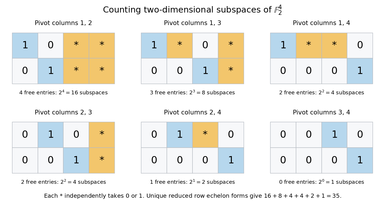
For $n=4,k=2,q=2$, there are $15\cdot 14=210$ ordered independent pairs. Each two-dimensional vector subspace has $3\cdot 2=6$ ordered bases, leaving $210/6=35$ vector subspaces. There are only $\left(\genfrac{}{}{0ex}{}{4}{2}\right)=6$ coordinate-selected vector subspaces; most of the 35 also contain vectors combining coordinates.

A unique reduced row echelon form gives another count. Its six possible pivot-column patterns have $4,3,2,2,1,0$ freely chosen entries. Each free entry lies in ${\mathbb{F}}_2$, giving $16,8,4,4,2,1$ vector subspaces, respectively. The diagram fixes the zero entries required to make each pivot the first nonzero entry in its row and the only nonzero entry in its column. Different choices describe different row spaces.

The Young diagrams of partitions in a rectangle with at most $k$ rows and at most $n-k$ cells in each row correspond to the lattice paths in the lattice-path interpretation of Gaussian binomial coefficients. Read the shaded row lengths from top to bottom; the result is a nonincreasing list of nonnegative integers. This bijection preserves the number $|\lambda |$ of cells.

In a two-by-two rectangle, the possibilities are the empty integer partition, $(1)$, $(2)$, $(1,1)$, $(2,1)$, and $(2,2)$. Their sizes are $0,1,2,2,3,4$, giving $G_{4,2}(t)$. In particular, there are two allowed diagrams of size two, explaining the middle coefficient.^[ref]

Use lattice paths with $k$ north steps and $n-k$ east steps, beginning at $(0,0)$. Let $A(P)$ be the sum of the horizontal coordinates of its north steps, equivalently the number of unit cells to their left inside the $k$-by-$(n-k)$ rectangle. A north step in zero-based word position $j_i$ has $i-1$ earlier north steps, so its horizontal coordinate is $j_i-(i-1)$. The Gaussian binomial coefficient recurrence therefore counts these lattice paths with weight $t^{A(P)}$.

For $n=4,k=2$, the words NNEE, NENE, NEEN, ENNE, ENEN, EENN have respective areas $0,1,2,2,3,4$. The word NEEN contributes $t^2$ because the two north steps occur at horizontal coordinates zero and two. These paths never move south or west; allowing such extra steps would change the collection being counted.

For $n\ge 1$ and $1\le k\le n$, the displayed recurrence relation uses $G_{n,0}(t)=1$ and $G_{n,k}(t)=0$ when $k<0$ or $k>n$. At $t=1$ it becomes Pascal's identity.

An exact weighted-subset formula isThe exponent measures how far the selected positions lie beyond the earliest possible choices $0,\dots ,k-1$. Split the subsets according to whether they contain $n-1$. Those without it give $G_{n-1,k}(t)$; deleting it from those with it removes exactly $n-k$ from their exponent. This gives the displayed recurrence relation, explaining why it builds polynomials with nonnegative integer coefficients.

The Rayleigh range of a fundamental Gaussian beam in vacuum is the positive axial distance from the beam waist at which its radius grows from $w_0$ to $\sqrt{2}{w}_0$. Thus its contour area doubles and its peak irradiance halves. Within $|z|\le z_R$, the radius stays at most $\sqrt{2}{w}_0$; for $|z|\gg z_R$, beam divergence dominates. At fixed vacuum wavelength, the Rayleigh range scales quadratically with the beam waist radius. The formula here uses the vacuum wavelength, not an unlabelled wavelength in a material.

The beam waist is the narrowest cross-section of a freely propagating Gaussian beam. Its radius $w_0$ uses the wave amplitude $1/e$, or light intensity $1/e^2$, convention; its diameter is $2w_0$. Specifying a “spot size” without saying radius or diameter can introduce a factor-of-two error. Within the scalar paraxial approximation, the wavefront at the beam waist is planar. The minimum radius sets both the Rayleigh range and the far-field beam divergence.

For uniform charge density ${\rho }_e=3Q/(4\pi R^3)$, Gauss's law gives the interior electric field $E={\rho }_{e}r/(3{\epsilon }_0)$. Integrate its vertical force density ${\rho }_e^{2}z/(3{\epsilon }_0)$ over the upper hemisphere: $\int zdV=\pi R^4/4$. Internal pair forces in that hemisphere cancel, so its net force is exactly the force from the lower hemisphere. The result is upward and has magnitude $3Q^2/(64\pi {\epsilon }_0{R}^2)$.

In static time times round three-dimensional hyperbolic space of curvature radius $R$, a geodesic sphere has area $4\pi R^2{\sinh }^2(\xi /R)$. The Gauss law therefore gives the displayed radial field. It approaches the flat-space inverse-square field near the charge and falls exponentially at large geodesic distance. The curvature changes the area of a sphere, not the conserved flux.

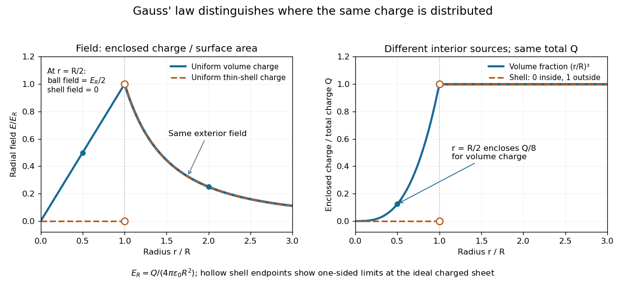
Place the same positive electric charge $Q$ uniformly on the sphere of radius $R$, with no external field. Every concentric interior Gaussian surface encloses zero charge; spherical symmetry then makes the interior electric field zero. Outside, it is again $Q/(4\pi {\epsilon }_0{r}^2)$. At $R$, the inner and outer limits differ by $Q/(4\pi {\epsilon }_0{R}^2)=\sigma /{\epsilon }_0$, with surface charge density $\sigma =Q/(4\pi R^2)$. The ideal surface charge makes the field discontinuous, so the plot displays one-sided limits rather than assigning a single field value on the charged sheet. An isolated charged conducting sphere in electrostatic equilibrium realizes this exterior/interior pattern.

Distribute a positive electric charge $Q$ uniformly through a closed ball of radius $R$ in vacuum, with no external field. Its volume charge density is $3Q/(4\pi R^3)$. For $0<r<R$, the enclosed fraction is $(r/R{)}^3$. Applying Gauss's law on a concentric Gaussian surface givesThe electric field grows linearly inside and decays as an inverse square outside. With $E_R=Q/(4\pi {\epsilon }_0{R}^2)$, its values at $r/R=1/2,1,2$ are $E_R/2,E_R,E_R/4$. The field vanishes at the centre by spherical symmetry and is continuous at the surface because this ideal volume distribution has no singular surface layer. Its interior behavior differs from a conductor in electrostatic equilibrium, where mobile charge redistributes.

For a minimal surface, the shape operator has eigenvalues $k,-k$, so $⟨dN(v),dN(w)⟩=k^2⟨v,w⟩$. Conversely this metric identity only implies that the two principal curvatures have equal squares. A sphere has equal nonzero principal curvatures and satisfies the identity while having nonzero mean curvature. The distinction is between opposite and equal signs, not equality of magnitudes.

Radially project a convex polyhedron from an interior point onto the unit sphere and triangulate each face without adding vertices. There are $T=2E-2F$ spherical triangles. The Gauss-Bonnet theorem gives each area as angle sum minus $\pi$. Summing angles around the projected vertices gives $2\pi V$, while the total area is $4\pi$. Thus $4\pi =2\pi V-\pi T$, proving the formula. Convexity guarantees that the projected triangles cover the sphere without overlaps of interiors.

For the conformal metric with $g_{0i}=-a^2{\partial }_{i}B$ and trace-free scalar spatial shear $E_{ij}=({\partial }_i{\partial }_j-{\delta }_{ij}{\nabla }^2/3)E$, the passive coordinate change $\tilde{\eta }=\eta +T$, ${\tilde{x}}^i=x^i+{\partial }^{i}L$ gives the displayed rules and $\tilde{\varphi }=\varphi +\mathcal{H}T+{\nabla }^{2}L/3$. The combination $C=\varphi +{\nabla }^{2}E/3$ changes by $\mathcal{H}T$, while $B+v$ changes by $T$. Hence $\mathcal{R}=-C+\mathcal{H}(B+v)$ is the comoving curvature perturbation in this sign convention.