
Past exam of the mathematics course of the University of Cambridge 2006 iii Paper 43 4 Solution Created 2026-10-03 Updated 2026-10-14
Let be the total exposure, and define the prior distribution expected value, prior variance and average binomial noise bySince the prior distribution has a probability density function on , and . All relevant moments exist because the parameter and observations are bounded. The binomial distribution givesThe law of total expectation, law of total variance and law of total covariance consequently yieldIn particular, conditional independence of the annual observations does not imply unconditional independence: they share the uncertain parameter.
To derive the optimal credibility estimate among affine functions of the observations, put and write . The conditional errors have zero conditional expectation, conditional variance , and zero pairwise conditional covariances. They are also uncorrelated with every integrable function of . Therefore the joint mean squared error isFor fixed slopes, the first term is uniquely minimized by . For fixed sum , the Cauchy-Schwarz inequality giveswith equality exactly when . Thus the remaining optimization is the strictly convex quadraticIts derivative vanishes at . Consequently the Bühlmann–Straub credibility estimate isThe individual coefficients are and . The strict quadratic minimizations establish global optimality and uniqueness, not just necessary equations. Here is the variance of hypothetical means, is the expected process variance, and is the Bühlmann–Straub credibility factor. More exposure gives more weight to the observed claim fraction. Since , the estimate remains between the observed pooled fraction and the prior expected value. If one separately permits a degenerate prior, leads to the constant estimate , interpreted as .
For the uniform distribution prior on ,With two years, put and . Then andTo compare with the Bayes estimator under squared error loss, use conditional independence to multiply the two binomial likelihood functions. Terms independent of cancel on normalization, and the uniform prior makes the posterior density proportional to . Hence Beta-binomial conjugacy givesFinally, for an arbitrary reported value , conditional quadratic loss decomposes asThe unique minimum is the posterior mean. Therefore the affine credibility estimate and the exact Bayesian estimate coincide in this case. The agreement illustrates exact beta-binomial credibility with unequal exposures; for a general prior distribution, minimizing over affine functions of the observations need not recover the unrestricted posterior mean.
Past exam of the mathematics course of the University of Cambridge 2006 iii Paper 43 3 Solution Created 2026-10-03 Updated 2026-10-14
In the classical risk model, the insurer's surplus iswhere is initial capital, is a Poisson process of rate , and the claim sizes are positive independent and identically distributed random variables with expected value , independent of the claim-arrival process. Premium flows in at constant rate . A positive relative safety loading meansso premium income exceeds the expected claim cost per unit time. The ruin stopping time is , with if ruin never occurs, and the ultimate ruin probability is .
Assume the stated positive adjustment coefficient exists and that the claim moment-generating function is finite at . The Lundberg inequality isHere is a proof, including the stopping argument. By conditioning on the Poisson distribution of , the random-sum transform identity givesThe adjustment coefficient equation is . Consequently the exponential surplus martingalehas expected value one at every finite time. More strongly, the claim process has independent increments, so for ,Thus is a nonnegative continuous-time martingale for the filtration generated by arrivals and claim sizes. For a fixed finite horizon , the optional stopping theorem at the bounded stopping time gives . This bounded use is legitimate: the stopped values belong to the closed martingale on given by conditional expectations of the integrable variable .
On , the surplus is negative, and therefore . By nonnegativity on the complementary event,The ruin events increase to as increases, so continuity of probability gives the claimed Lundberg inequality. No expectation identity at the unbounded stopping time is needed. Positive loading by itself does not guarantee a positive adjustment coefficient for every claim law; the existence assumption is used here.
For the exponential distribution of claim sizes, for . Substitution in the adjustment coefficient equation givesDiscard the zero root and divide by . The unique positive solution iswhich lies strictly inside the finite-transform domain.
For deterministic claim sizes, the claim moment-generating function is . Define . It satisfies , , , and as . Thus its strict convexity gives exactly one positive zero , with for .
Put . Since , we have . HenceIt follows thatThus the deterministic-claim Lundberg inequality provides a smaller upper bound at positive capital; at zero capital both bounds equal one. This is a special case of deterministic claims maximize the adjustment coefficient at fixed mean and loading: fixing the mean and loading, variability lowers the exponential decay coefficient relative to deterministic claims. The ordering of these upper bounds alone is not a proof that the actual ultimate ruin probabilities are ordered.
Past exam of the mathematics course of the University of Cambridge 2006 iii Paper 43 2 Solution Created 2026-10-03 Updated 2026-10-14
The claim-size exponential distribution has expected value and moment-generating functionConditional on , independence makes the aggregate moment-generating function equal to . Averaging over the Poisson distribution of the count givesPut . For fixed intensities, independence between risks givesThis is precisely the transform of a compound Poisson distribution. Indeed the addition of independent Poisson random variables makes the total count Poisson distributed with parameter , and every claim in the pooled portfolio has the same exponential distribution. Thus the portfolio aggregate is compound Poisson with intensity and exponential claim sizes of mean .
Now regard the individual intensities as independent gamma distributed quantities, with shape and rate . Their moment-generating functions are for . Multiplying these transforms proves additivity of independent gamma distributions with a common rate:Conditional on the individual intensities, the total count has Poisson distribution with parameter . Because this conditional law depends only on their sum, it is also the law of conditional on . Integrating its probability mass function against the gamma distribution density yieldsThus the total count has a negative binomial distribution with shape and success probability , using the convention that counts failures before the specified number of successes. Its probability generating function is .
Conditional on , the claim sizes retain their common exponential distribution and the amount has a compound Poisson distribution of intensity . Therefore the unconditional amount has a compound mixed Poisson distribution with gamma mixing intensity of shape and rate . To make the mixture explicit, average the conditional aggregate moment-generating function:The displayed domain ensures both the severity transform and the intensity transform are finite. The mixing distribution describes the Poisson intensity, not the claim sizes. In particular, the aggregate has an atom at zero of mass .
Past exam of the mathematics course of the University of Cambridge 2006 iii Paper 43 1 Solution Created 2026-10-03 Updated 2026-10-14
Write , and for the three probability generating functions. Since both the claim count and every claim size are positive, . Conditioning on the count and using independence gives the random-sum transform identityThe crucial point is that the count recurrence begins at . Multiplying it by and summing, we obtainConsequently . The chain rule applied to the aggregate probability generating function therefore givesThese identities hold inside the unit disk, or as identities of formal power series. Since , every coefficient of the composition depends on only finitely many count probabilities.
Compare the coefficient of . The product contributes , and contributes . HenceThe required aggregate recursion for zero-truncated Panjer counts is initialized by and , and for every it isThe empty sum at is zero. Every term on the right is known or has a smaller aggregate index. Omitting would incorrectly apply the usual Panjer recursion with a zero initial value, producing zero for every aggregate probability.
For the zero-truncated Poisson distribution, for , so , and , with . ThusAs a direct probability generating function check, and therefore ; differentiation reproduces this recursion.
Past exam of the mathematics course of the University of Cambridge 2006 iii Paper 42 6 Solution Created 2026-10-03 Updated 2026-10-20
Let . Near the interior minimum, Taylor expansion givesOn the scale , the leading exponent is and . If the integral is localized at this minimum, the rescaled integration endpoints tend to infinity in both directions, so the Gaussian integral gives Laplace's method:Formally expanding the cubic term gives an order- correction odd in , whose Gaussian integral is zero. Quartic terms and the square of the cubic term produce the order- correction. Sufficient smoothness near the minimum and control of the exterior integral justify this formal calculation.
The printed local assumptions alone do not guarantee localization. A useful localization condition for Laplace's method is that outside each sufficiently small fixed neighbourhood of , for some , and that for some . For , the exterior contribution is at mostwhich is exponentially smaller than the displayed local term. To see why something of this kind is needed, take on . Its unique minimum is at zero and , yet on we have . This boundary interval alone contributes at least , dominating the proposed local approximation. The Laplace formula therefore has its usual implicit tail assumption, rather than following from uniqueness of the interior minimum alone.
For the gamma function, set to obtainHere has its unique minimum at , with and . It tends to infinity at both endpoints, and its integral is finite for positive exponents, so localization holds. Laplace's method yields Stirling's formula:
For a prior density and independent observations, Bayes' theorem writes the desired posterior expectation as a ratio of integrals:Suppose the log-posterior kernel has a unique concentrating interior mode , with curvature of order , and the smoothness and tail conditions hold for both integrals. Expanding quadratically gives a common Gaussian factor . Replacing the smooth amplitude by givesThis approximation does not require to be positive: it treats as an amplitude, without taking its logarithm. For more accuracy, expand the amplitude and the cubic term in the log-posterior kernel. With , the Gaussian moments are and . Terms multiplying cancel between numerator and denominator; the two remaining first corrections areunder the stronger smoothness, derivative-scaling and integrability assumptions needed for this expansion. The first term accounts for the curvature of the amplitude and the second for posterior skewness. This is posterior expectation by Laplace approximation. If there are several modes, boundary modes, or nonconcentrating tails, the appropriate separate contributions must be included; a single interior Gaussian approximation cannot then be assumed.
Past exam of the mathematics course of the University of Cambridge 2006 iii Paper 42 5 Solution Created 2026-10-03 Updated 2026-10-14
Write . The kernel density estimator with bandwidth isSufficient conditions are that be a nonnegative symmetric probability density function with and finite nonzero second moment , and that , . Symmetry and the second-moment assumption give . The expectation is a convolution:Taylor's theorem with integral remainder givesThe zeroth-order term integrates to , and the first-order term vanishes. The second derivative is bounded and continuous, so dominated convergence, with dominating function proportional to , yieldsCombining this with the supplied leading variance gives the asymptotic mean squared errorWhen and , its derivative is . It changes sign exactly once, giving the pointwise optimal kernel bandwidthPositivity of is needed for this positive interior optimum. The printed condition alone does not ensure it. For instance, is a normalized bounded probability density function with bounded continuous square-integrable second derivative, but and . At this point the displayed leading variance vanishes and the two-term AMSE has no positive interior minimizer; finer variance terms are needed to determine an appropriate bandwidth. The formal formula there gives zero, which does not satisfy the bandwidth assumptions.
For integrated error, the same expansion holds in : translation continuity of applied to the integral remainder givesIndeed Minkowski's integral inequality bounds the norm of the difference, divided by , by the integral of ; each translated difference tends to zero and is bounded by . This proves the claimed integrated bias expansion without assuming a uniform pointwise remainder over the whole real line.
If , direct integration of the variance givesThe last term is because is bounded and integrable, hence square integrable, and convolution with a probability density function does not increase its norm. It is negligible compared with . Thus the asymptotic mean integrated squared error and its minimizer areHere : otherwise the continuous second derivative vanishes everywhere, making affine, impossible for a probability density function on the whole real line.
Now take the standard normal density . Differentiation gives . Gaussian integration givesThe kernel constants cancel from the bandwidth ratio. At ,Put . The logarithmic derivative of is . On the function increases, giving its minimum at , with value one. On it decreases up to and then increases, giving its minimum . Thus the global minimizers are , and the normal-density local-to-global bandwidth ratio isThe ratio diverges at the two inflection points , where the second-order pointwise bias approximation vanishes and needs a higher-order replacement.
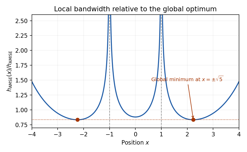
Normal-density pointwise bandwidth relative to the integrated-error optimum; minima at plus and minus square root of five
. Details. 
Past exam of the mathematics course of the University of Cambridge 2006 iii Paper 42 3 Solution Created 2026-10-03 Updated 2026-10-14
For a nondegenerate distribution function , membership in its maximum domain of attraction means that there exist such thatat every continuity point of . A max-stable distribution satisfies: for each positive integer , there exist such that . Thus a maximum of independent copies has the same probability distribution after a change of location and scale.
Suppose first that . For fixed , the distribution functions have the two nondegenerate limitsThe given convergence-of-types result supplies constants such that . Equality extends from continuity points to all points by right continuity. Substitute to obtain , which proves max-stability with . Conversely, if is max-stable, take and its max-stability constants for . Then exactly for every , proving . Therefore the maximum domain of attraction is nonempty exactly when is max-stable.
For the particular logarithmic tail, complete the distribution function by taking for . Let be the unique solution of , and take . Equivalently , including with . For each fixed , eventually , andHere follows directly from its defining equation. Since as , it follows that . For , the probability is zero. ConsequentlyThis is the shape-one Fréchet distribution, and the calculation proves the limit at every real without needing a regular variation theorem.
The function is strictly increasing on . For every integer , , so . The defining equation now gives . Taking logarithms yields , whose right side is positive, soMultiplying by and squeezing gives . Slutsky theorem applied to the normalized sample maximum therefore gives the simpler logarithmic-tail Fréchet normalization
Past exam of the mathematics course of the University of Cambridge 2006 iii Paper 42 2 Solution Created 2026-10-03 Updated 2026-10-20
Write and for the individual and total score functions. Under the usual regularity assumptions, and , the nonsingular per-observation Fisher information matrix. The central limit theorem and weak law of large numbers giveRearranging the stipulated score expansion, including its remainder, givesSlutsky theorem therefore proves the asymptotic normality of a maximum likelihood estimator:A consistent plug-in Fisher information matrix yields the Wald statistic . Under the null hypothesis, , so a test of asymptotic size rejects when exceeds the quantile of that chi-squared distribution. A consistent observed Fisher information matrix gives the same limiting test.
With an -dimensional parameter of interest and nuisance parameter , partition accordingly. The marginal asymptotic covariance matrix of is the block of , whose inverse is the efficient informationThus the nuisance-adjusted Wald statistic is , with limiting null distribution . Using alone is generally incorrect when the nuisance parameter is estimated; it is valid when the cross-information vanishes.
For the Inverse Gaussian distribution in this problem, expand the exponent to obtain the log likelihood, up to terms independent of both parameters,Its score functions areFor each positive , the first score changes sign from positive to negative at , so this is the global maximizing mean parameter of an exponential family. Substituting it in the second score givesThe reciprocal function is strictly convex, so the denominator is positive for a nonconstant sample. The profile log likelihood is strictly concave in and tends to minus infinity at both endpoints, proving this is a maximum. Under continuous model sampling, a sample of size at least two is nonconstant almost surely. For a constant sample, including a one-observation sample, no finite joint maximum-likelihood estimator exists: the likelihood increases without bound as at .
For one observation, differentiating again and using givesThis parameter orthogonality proves that estimating does not reduce the efficient information for . The Wald statistic has the same algebraic form in the two cases:Using information evaluated at instead is another first-order equivalent convention.
The printed claim of coincidence needs a first-order interpretation. Known and unknown need not give numerically identical Wald statistics, because their maximum-likelihood estimators differ. With known, direct maximization givesFor example, observations and known give and . At , the displayed Wald convention gives and , respectively. Thus exact equality is false. Under the null hypothesis, however, , hence . Their centered, standardized estimates differ by , so their Wald statistics differ by . This is the valid asymptotic coincidence supplied by inverse Gaussian shape estimation and nuisance orthogonality.
Past exam of the mathematics course of the University of Cambridge 2006 iii Paper 42 1 i Created 2026-10-03 Updated 2026-10-14
Past exam of the mathematics course of the University of Cambridge 2006 iii Paper 41 5 a Created 2026-10-03 Updated 2026-10-14
Past exam of the mathematics course of the University of Cambridge 2006 iii Paper 41 4 Solution Created 2026-10-03 Updated 2026-10-14
For independent binomial distributions, the log-likelihood, up to known binomial coefficients, isThe saturated statistical model maximizes each term at . Under the logit link, the fitted probabilities are . Subtracting the fitted log-likelihood from the saturated log-likelihood gives the binomial devianceA zero-count summand uses the continuous convention . For the restricted model, replace by to obtain . Since the saturated likelihood cancels, is the likelihood-ratio test statistic. For the nested restriction setting coefficients to zero, Wilks theorem gives the asymptotic chi-squared distribution under regularity and an interior true parameter; reject for a large difference.
For the six anther cells, gives a common success probability, gives a separate probability for each storage condition, gives a common intercept and a log-force slope, and gives storage-specific intercepts with a common log-force slope. Their parameter counts are , so their residual statistical degrees of freedom are . In , storage has a constant effect on log odds; multiplying force by multiplies the odds by in either storage group.
The relevant nested likelihood-ratio tests at the level are:
- Adding storage to gives on one statistical degree of freedom, with .
- Adding log-force to gives on one statistical degree of freedom, with .
- Adding log-force to the storage model gives on one statistical degree of freedom, with .
- Adding storage to the log-force model gives on one statistical degree of freedom, with .
- Adding both terms to gives on two statistical degrees of freedom, with .
The two two-parameter models and are not nested, so their deviance difference has no ordinary nested chi-squared distribution calibration. The preferred parsimonious model is , with a storage effect and no log-force effect. Its deviance goodness-of-fit test is acceptable: on four statistical degrees of freedom. The common-probability model also passes its separate goodness-of-fit comparison, , but this does not contradict the relative evidence for adding storage: the two tests assess different null hypotheses. These are large-sample approximations; sufficiently large expected successes and failures, not merely the number of anthers, underpin their calibration.
Past exam of the mathematics course of the University of Cambridge 2006 iii Paper 41 3 Solution Created 2026-10-03 Updated 2026-10-14
The Poisson distribution mass function isIt is an exponential dispersion family of order one withIndeed, and . A generalized linear model specifies independent random variables from a response exponential family, together with a linear predictor and a link function relating it to the response mean. The Poisson canonical link is .
For the insurance counts, let class and merit be the reference levels in a regression factor. The fitted Poisson regression assumesThe insured exposure is known; its logarithm is an offset, not a coefficient to estimate. The model has eight free mean parameters and fixes the dispersion parameter at one. It assumes additive class and merit effects on the log-rate scale, hence multiplicative effects on the rate scale without a class-by-merit interaction.
Apart from constants independent of the parameters, the log-likelihood isDifferentiating gives the Poisson regression margin-matching score equationsThus the fitted totals equal the observed totals in each class and merit category, including the reference categories by subtraction. In design matrix notation these equations are . Fisher scoring solves them iteratively; the reported three iterations describe the numerical fit, not an additional statistical result.
The regression intercept gives the baseline fitted claim rate per insured car year. The merit rate ratios, relative to merit at the same class, areThe class rate ratios, relative to class at the same merit, areEach predicted cell rate is the baseline rate times its class and merit multipliers. The output's coefficient-to-standard error ratios are asymptotic normal Wald test statistics under the fitted Poisson regression, despite the software label “t value”; there is no estimated Gaussian residual scale in this model. All nonreference effects have very large absolute ratios.
The null Poisson deviance is on nineteen statistical degrees of freedom; adding the seven factor coefficients reduces it by . But the final Poisson deviance is still on twelve statistical degrees of freedom, and the deviance residuals include values near and . These are far beyond what a well-fitting unit-dispersion model would normally produce. The additive Poisson model fits substantially better than a common rate, but remains grossly inadequate. A class-by-merit interaction, overdispersion, or statistical dependence between claims could contribute; the summary alone does not distinguish these explanations. Its very small nominal standard errors and formal Wald tests rely on the rejected model, so improved mean structure and error assumptions are needed before treating them as reliable uncertainty assessments.
There are unlisted articles, also show them or only show them.