
Past exam of the mathematics course of the University of Cambridge 2006 iii Paper 41 2 Solution Created 2026-10-03 Updated 2026-10-14
A factor is a categorical predictor whose levels distinguish experimental conditions. Two factors have a statistical interaction when the effect of changing one depends on the other's level. For cell means , absence of an interaction means ; equivalently, is independent of .
Index thickness by , temperature by , wash by and replication by . The full factorial design has the normal linear modelThe errors are independent with a common positive variance. Sum-to-zero constraints in each factor index, or the displayed treatment coding, identify the mean coefficients. This full model allows an arbitrary mean in each of the sixteen cells.
The missing statistical degrees of freedom, in the output order, are . The first seven entries total fifteen; with the regression intercept there are sixteen mean coefficients among thirty-two observations, leaving sixteen residual statistical degrees of freedom. Balanced factorial orthogonality makes the term sums of squares in ANOVA independent of their ordering.
All terms involving wash have nonsignificant individual F-tests, and it is useful to test their removal jointly. The reduced model omits twelve mean coefficients. Its residual sum of squares is , compared with for the full model, so the nested-model F-test givesThere is no detected wash effect over the four tested durations. Removing its main effect and all its interaction terms respects the principle of marginality. Retaining the very large thickness-by-temperature interaction is essential: the thickness effect changes substantially with temperature.
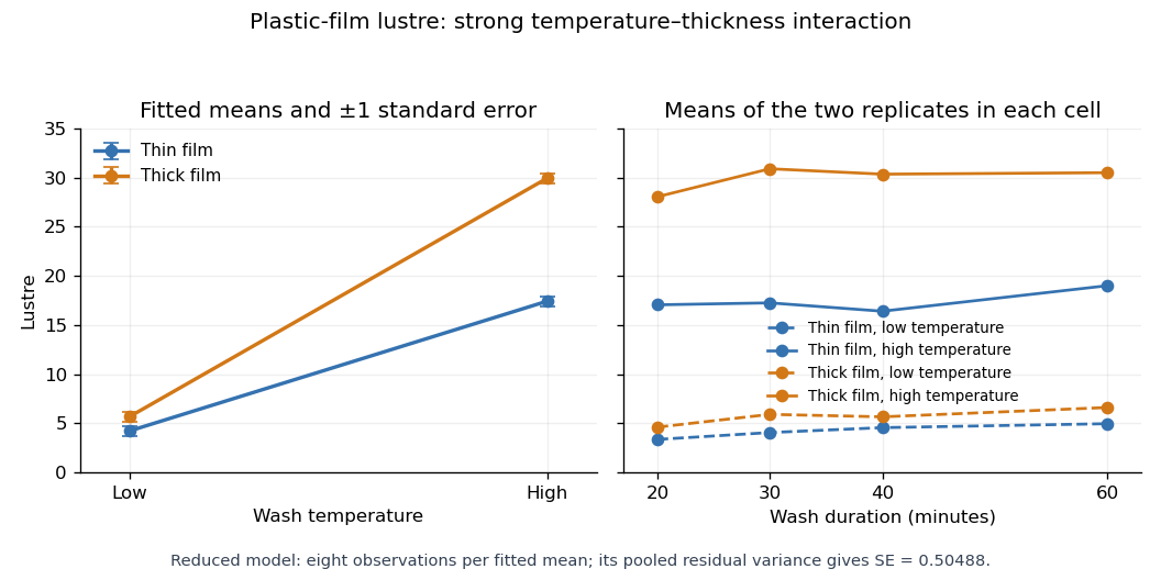
With numeric indicators , treatment coding expresses the reduced fitted mean asThus the thin/low, thick/low, thin/high and thick/high fitted means are , respectively, at every wash level. Each is the sample mean of eight observations. The equal-cell replication variance formula therefore givesAlternatively, use the variance of a fitted regression mean with : . Individual coefficient standard errors cannot simply be added; their covariances enter the fitted-mean calculation.
Increasing temperature raises fitted lustre by for thin film and for thick film. Increasing thickness raises it by at low temperature and at high temperature. Their difference, , is the estimated interaction contrast; its standard error is , giving on twenty-eight statistical degrees of freedom. The interaction plot shows this strong departure from parallel mean lines, while the wash panel shows the much smaller variation across wash durations. Neither the nonsignificant wash test nor the plot proves that its true effect is exactly zero.
Past exam of the mathematics course of the University of Cambridge 2006 iii Paper 41 1 Solution Created 2026-10-03 Updated 2026-10-14
Minimizing the residual sum of squares gives the least-squares normal equations . Since the design matrix has full column rank, has a matrix inverse, soThe sampling distribution follows because a linear transformation of a multivariate normal distribution is again a multivariate normal distribution. Its expectation is , and its covariance matrix is .
The hat matrix is . It is the orthogonal projection matrix onto the column space of : , and . Thus the regression residuals are , withThis is fitted-residual orthogonality. The vectors are jointly normal, so independence of uncorrelated jointly normal variables strengthens both zero-covariance statements to independence.
For the quadratic linear regression, the columns of the design matrix are . The replicated design givesFor , the variance of a fitted regression mean is , henceWriting , this is the quadratic . Its derivative vanishes at ; it decreases before that point and increases afterwards. Therefore the maximum is at , and the minimum is at .
At , and the expected yield is . The unbiased residual variance estimate is . By Cochran's theorem, independently of , giving the Student t confidence intervalThe interval estimates the expected yield, so it uses the variance of a fitted regression mean without an additional future-observation error term. The supplied summary determines the half-width but does not give a numerical value of .
Past exam of the mathematics course of the University of Cambridge 2006 iii Paper 40 4 Solution Created 2026-10-03 Updated 2026-10-14
Use column vectors for dollar holdings and put , and . The normalized state-price density isThe vector is the market price of risk. The density defines an equivalent risk-neutral measure, under which is Brownian motion and every stock has drift . A terminal claim with finite state-price cost is priced at . Nonsingularity of and the natural Brownian market information make this a complete market; in particular the optimal nonnegative payoff below can be replicated.
Let and . Apply the Itô formula to each log price, whose return variance is :Summing and dividing by proves the geometric stock index formulaThus , where . The factor applies to the whole bracket. The geometric average need not itself be a self-financing portfolio; its instantaneous drift is .
If is the dollar amount invested in stock , the bank account holds . The self-financing portfolio equation isEquivalently, gives . For share-holding notation replace by times the number of shares.
Static expected utility maximization uses the terminal budget . Since is an exogenous positive benchmark, differentiating in gives . An interior Lagrange multiplier for the budget therefore givesFor CRRA utility, write . Since , solving this marginal equation givesEvery positive lognormal moment is finite here, so the budget determines the constant uniquely. PutThenThis is also a sufficiency condition: concavity gives , and taking expectations and using the budget inequality proves global optimality.
To find the whole optimal process, set andSince , the moment-generating function of a normal distribution givesPricing the terminal payoff yields the explicit benchmark-relative power-utility portfolio wealthIts proportional diffusion coefficient is . Since the wealth diffusion coefficient for dollar fractions is , replication requiresUsing gives the requested fixed proportions:The drift matches the self-financing portfolio equation as well. Indeed, , so the drift of from the explicit formula isConsequently an equivalent form of the solution isThe bank account fraction is , with negative values representing borrowing. The first stock term is ordinary power-utility risk exposure, while the second hedges the random benchmark. At the logarithmic limit the benchmark term disappears, consistently with .
Past exam of the mathematics course of the University of Cambridge 2006 iii Paper 40 3 Solution Created 2026-10-03 Updated 2026-10-14
Assume, as in the Bayesian model, that the unknown drift is independent of the driving Brownian motion, with known positive prior precision . Recover the observed signal from the positive stock price:For a fixed time , the centered observed path is a Brownian bridge independent of : it is independent of the prior and has zero covariance with in their joint Gaussian law. Thus the whole observed history has the same posterior information about as its endpoint. This proves Brownian endpoint sufficiency for a constant drift rather than assuming it.
The likelihood of that endpoint, as a function of , is proportional to . Multiplying by the normal distribution prior and completing the square gives the Gaussian Brownian drift filterDefine the observed innovation process . It is a continuous observed-filtration martingale: for , independence of future noise and the tower property of conditional expectation give , so the conditional mean of its increment vanishes. Its quadratic variation is , since subtracting the finite-variation drift from does not change quadratic variation. The Lévy characterization of Brownian motion makes an observed-filtration Brownian motion. Differentiating the posterior mean givesConversely, the last equation determines from with deterministic coefficients and known initial value, and . Thus the observed and innovation filtrations coincide, supplying the natural Brownian information needed for replication. Consequently the observed stock dynamics are . Its observed market price of risk is , and its normalized state-price density solvesThe posterior mean is unbounded, so bounded-coefficient Novikov condition reasoning from Question 2 is not available automatically. A direct finite-horizon argument supplies true pricing. Relative to driftless Wiener measure for , the Bayesian mixture has observation densityA law with observation drift instead has density . ThereforeThis is the finite-horizon pricing density for Gaussian drift learning. The ratio changes the physical observed law into a genuine probability law, hence has mean one. Indeed, differentiation of the explicit likelihood, using , givesThe Itô formula therefore gives , agreeing with the stochastic exponential above. Under this pricing law the stock drift is .
For logarithmic utility, terminal marginal utility is . The state-price budget constraint and the marginal condition imply and . Since is constant, its conditional-expectation pricing process is constant as well. Thus the entire optimal wealth process isIndeed, for any other nonnegative admissible terminal wealth , the elementary inequality givesThis directly verifies optimality. Expected candidate log wealth is finite because and its time integral is finite on every fixed horizon. Applying the Itô formula to givesThe observed self-financing portfolio with risky dollar fraction has diffusion coefficient . Matching the coefficients proves the log-optimal investment with Gaussian drift learning ruleThe remaining dollars are held in the bank account; the fraction may be negative or exceed one because the question imposes neither short-sale nor borrowing restrictions.
Past exam of the mathematics course of the University of Cambridge 2006 iii Paper 40 2 Solution Created 2026-10-03 Updated 2026-10-14
Use for the dollar amount invested in the stock; the number of shares is . The bank account contains dollars. With no intermediate consumption, the self-financing portfolio equation isIf instead denotes share holdings, replace each dollar here by . The equation says that trading only reallocates existing portfolio wealth; gains come from cash interest and stock returns.
For the standard unconstrained complete-diffusion formulation, assume the completed natural Brownian filtration, initial wealth , and nonnegative admissible wealth. Define the market price of risk . The boundedness assumptions make bounded. The state-price density normalized at zero isIts money-market-adjusted process is a true martingale by the Novikov condition. Under , the Girsanov theorem gives as a Brownian motion, and the discounted stock has zero drift.
The Itô product rule applied to the wealth equation givesFor nonnegative admissible wealth this is a nonnegative local martingale, hence a supermartingale. Therefore every affordable terminal payoff satisfies the state-price budget constraint . Nonzero volatility and the Brownian martingale representation theorem allow replication of nonnegative claims with finite state-price cost.
For a differentiable strictly concave utility function with the usual conditions ensuring an interior integrable optimizer, put , the inverse marginal utility. Pointwise maximization of givesThe second equation determines the positive constant . To prove optimality, use the concave supporting-tangent inequality:Taking expectations and using the budget bound proves that the candidate dominates every admissible affordable payoff, whenever the utility expectations are well defined. This is the complete-market terminal utility optimizer.
The actual wealth and dollar portfolio are as explicit as general adapted coefficients permit. LetThe Brownian martingale representation theorem, with localization if only integrability is initially known, gives . The dollar portfolio from a deflated wealth martingale isThe bank holds dollars. Equivalently, with , . These formulas need no unjustified differentiability of a value function with random coefficients.
The printed assumption that is only increasing and concave does not guarantee that the interior formula exists, or even that the optimal value is finite. In general replace the inverse formula by an affordable selectionwhere is the wealth domain; boundary choices or supporting slopes handle nondifferentiability. Existence, finite cost and replication still have to hold. A concrete obstruction is the unbounded linear terminal-wealth utility: take , , , and the Brownian filtration. Then . For , the bounded nonnegative claimis replicable, costs , and has . Thus there is no finite optimal expected utility under the literal utility hypotheses alone. Also, bounded coefficients do not ensure market completeness in an arbitrarily enlarged filtration containing untraded randomness; the full replication formula uses the Brownian market information assumption stated above.
Past exam of the mathematics course of the University of Cambridge 2006 iii Paper 4 6 Solution Created 2026-10-03 Updated 2026-10-14
For a cell in the Young diagram of , its hook of a Young diagram consists of that cell, the cells to its right in row and the cells below it in column . Its length isA removable rim hook is a connected border strip containing no square, whose removal leaves a Young diagram. Its leg length is the number of rows it meets minus one. The hook graph is the Young diagram labeled at each cell by ; here “graph” means this labeled array, not a graph of possible hook-walk moves.
Choose , pad with zeros and form the beta numbersThey are distinct nonnegative integers in decreasing order and recover . For they equal the first-column hook lengths, since . If is increased, old beta numbers shift upward by one and a new bead at zero is inserted.
For a prime-modulus partition abacus arrange the nonnegative positions in runners: position lies at level on runner , . Put beads at the beta numbers and leave the other positions empty. Replacing a bead at by a bead at a vacant removes a rim hook of length ; its leg length is the number of beads strictly between these positions. This follows by tracing the boundary of the diagram: bead positions record vertical steps and gaps record horizontal steps, and exchanging one bead and gap removes the intervening border strip. In particular a removable -hook is exactly a bead that can slide up one place on its own runner.
The partition core at modulus is the result of sliding beads up until there are no gaps above any bead on a runner. If runner initially has beads, its final occupied levels must be , independently of slide order. Thus its packed beta set, and hence its core partition of an integer, is unique. Increasing the number of beta numbers merely re-expresses the same boundary by shifting positions and adding the new initial bead; the packed configuration represents the same partition of an integer. This proves well-definedness both with respect to removal order and to the chosen padding. The number of slides isThe partition quotient components record how far each runner's beads lie above their packed positions, giving the hook-removal interpretation used in Question 5.
A block of a group algebra in characteristic for is a two-sided ideal for a primitive central idempotent , meaning a nonzero central idempotent that is not a sum of two nonzero orthogonal central idempotents. The identity is the sum of these block idempotents and the group algebra is their direct product. An indecomposable module belongs to when , equivalently every other block idempotent acts as zero. Indeed ; indecomposability makes exactly one summand nonzero.
The Nakayama block theorem, historically called the Nakayama Conjecture, statesEquivalently the ordinary characters assigned to one modular block have a common partition core at modulus . Its simple modules are the with regular having that core. Only cores for which is a nonnegative multiple of occur. The block weight is ; a core alone determines the block at this fixed degree.
One route to the proof separates the combinatorial core invariant from the algebraic center invariant. Let be the number of cells of residue . A length- rim hook has one cell of every residue: along its border strip the contents are consecutive integers. Therefore removal subtracts one from every . More precisely, choose the number of beta numbers divisible by and write the runner charges as . Reading the boundary, or adding a cell and checking its two changed beta positions, givesThe charges determine the packed runners and hence the core. For fixed , two equal cores have the same weight, so their full residue multisets are equal. Conversely equal residue multisets give equal charges and the same core. This establishesfor partitions of an integer of the same integer. The fixed-degree condition matters.
For the center invariant, use the commuting Jucys–Murphy elements , with . In the Young seminormal form basis, has eigenvalue equal to the content of the cell containing . A symmetric polynomial in them therefore acts on as the same scalar for every Young tableau: its value on the multiset of all contents of . The integral Specht lattice makes this a scalar identity before modular reduction, so modulo these central scalars depend only on the residue multiset, and every composition factor inherits them.
The substantive center theorem used in this proof is that the center of the symmetric-group algebra, integrally and over a field, consists of symmetric polynomials in the Jucys–Murphy elements. Centrality of elementary symmetric polynomials follows fromthe coefficients are central class-sum combinations. The reverse inclusion requires the integral triangular class-sum argument: expand symmetric monomials in the as products of transpositions, group the leading terms by reduced cycle type, and eliminate these leading class sums in the resulting unitriangular order. The integral coefficients, with no division by multiples of , are crucial; knowing the center only over would not prove the modular assertion. This is the central algebraic ingredient of this proof route.
Thus equal residue multisets yield equal characters of the entire modular center. Different residue multisets are separated already by the coefficients of the central polynomial : its scalar on the shape reduces to , whose unique factorization records the multiplicities exactly, even in characteristic . In a finite-dimensional split algebra, two simple modules are in the same block exactly when their central characters agree: the center of each block is local, while different block idempotents separate different blocks. It follows that equal cores give one block and different cores give distinct blocks. This proves both directions rather than just observing that core is constant on known blocks.
Finally, each ordinary Specht lattice has a single reduced central character, so all constituents of its reduction lie in that one block. Question 1 supplies every simple module and its label; the regular labels therefore identify all the simples in each core block. The constructions use integer coefficients and absolutely irreducible prime-field modules, so the block description descends to the arbitrary characteristic- field in the question. This completes the main steps of the block proof without presupposing semisimplicity in positive characteristic.
Past exam of the mathematics course of the University of Cambridge 2006 iii Paper 4 5 Solution Created 2026-10-03 Updated 2026-10-14
Use the induction product of symmetric-group characters: for , is the trivial character of , is the unit and for . Products mean induction of external tensor products. The determinantal form iswhere . Each determinant term is a virtual character of , because its indices sum to .
Here is a proof. The Frobenius characteristic map sends to the complete homogeneous symmetric function , and induction products to multiplication. By Young's rule its value on is the Schur function , the generating function of semistandard tableaux of shape . To identify that function with , work in variables and take starting points and ending points . A path from to has east and north steps; each east step at height has weight and each north step has weight one. Its east-step count is , so its weight sum is . Expanding the determinant sums signed systems of paths with permuted endpoints. For a system with an intersection, exchange the two tails after the first intersection. This preserves its monomial weight and reverses the endpoint permutation's sign, so all intersecting systems cancel in pairs. Nonintersecting systems necessarily have the identity endpoint permutation and correspond precisely to weak rows with strictly increasing columns, namely semistandard tableaux of shape . Their signs are positive. This proves , the Jacobi–Trudi identity, and injectivity of the Frobenius characteristic map gives the character formula above. The path sum may be taken in finitely many variables first and then stabilized, so no infinite formal sum is required in the argument.
A removable rim hook, or border strip, of length is a connected skew diagram of cells with no square, where removal leaves a partition of an integer. Its leg length is the number of occupied rows minus one. The Murnaghan–Nakayama rule statesA proof sketch follows directly from the alternant form of Schur functions. Multiply an alternant by . In each term one alternant exponent increases by . Equal exponents cancel; otherwise reordering the exponents contributes the sign of the number crossed. In the beta-set description, increasing one exponent is adding a -rim hook, and the number crossed is its leg length. Therefore . Taking its adjoint in the Hall inner product of symmetric functions, where Schur functions are orthonormal and power-sum symmetric polynomials have squared norm , reads off the value at a -cycle and the remaining cycle type. This gives the stated rule and explains its sign.
The printed shape is , of size 11; the converted TeX's is incorrect and would have the wrong size. There are two removable length-5 rim hooks. They leave with leg length 2 and with leg length 1. ThusThe staircase has no removable length-4 rim hook, so its term is zero. The unique removable length-4 rim hook of leaves and has leg length 1. The remaining length-2 rim hook in also has leg length 1, giving . HenceAs a separate determinant check, the only term whose row sizes can be unions of cycles of lengths is the transposition term with sizes . Its permutation character has value one and its determinant sign is negative.
Taking in the Murnaghan–Nakayama rule removes a single corner and every leg length is zero. Evaluating on a permutation fixing the distinguished point therefore givesThis is the restriction branching rule for a symmetric group; ordinary semisimple representation theory converts the character equality into a direct-sum decomposition. Frobenius reciprocity gives the corresponding add-one-cell induction rule.
For a positive prime , the weight of a partition at prime modulus , denoted , is the number of length- rim hooks removed in reaching its partition core , so . On a prime-modulus partition abacus write its partition quotient as and put , with . Removing a length- rim hook removes one corner from one quotient partition of an integer. Complete removal sequences therefore numberwhere is the hook product of a partition and . Each component's standard tableaux encode its possible removal orders, and the multinomial coefficient interleaves the components.
All these sequences have the same total sign . To see this, label the beads on each runner in their preserved order. Each slide crosses exactly the beads counted by its rim-hook leg. Its sign is the change in the total order of bead labels, and the product telescopes to the permutation from the initial ordering to the final packed-core ordering, independently of the slides chosen. Repeating the Murnaghan–Nakayama rule on the distinguished -cycles givesHere acts on the complementary letters; no -regularity hypothesis on is necessary. If its cycle type contains a part divisible by , the partition core character is zero, since its partition abacus admits no hook removal of a length divisible by . For the coefficient and sign are one.
Past exam of the mathematics course of the University of Cambridge 2006 iii Paper 4 4 Solution Created 2026-10-03 Updated 2026-10-14
Use the pair of partitions for a generalized Specht module convention appropriate to generalized Specht modules. Put and . Here is a sequence of nonnegative row lengths of total , and is a proper partition of an integer satisfying and . The row-length sequence is allowed to be a composition; it need not decrease. The first cells of row are marked. This construction is not an arbitrary pair of unrelated partitions of an integer and is not simply a skew diagram .
A word has type if it contains occurrences of . Read it from left to right. Every occurrence of is good; an occurrence of is good exactly when there have so far been more good occurrences of than good occurrences of . Otherwise it is bad. DefineThus is the set of all words of type , and consists of lattice words when is a proper partition of an integer. Marking the whole first row makes no difference because every is good.
For a Young tableau with row lengths , let permute labels within each column of its marked subdiagram, fixing all unmarked labels. Its generalized polytabloid and generalized Specht module areIn particular and . The Young tableau shape in this definition must be the row sequence .
We give the filtration argument, keeping its combinatorial and module-theoretic steps separate. Normalize , and if choose the first row with . Then . Define if ; otherwise the add branch is empty. Define by moving the unmarked tail of row into row :with other row lengths unchanged. Re-normalize the first marked row if necessary. The Basic Combinatorial Theorem supplies the counting and formal-character recursionsAt a terminal pair the formal term is . Thus the second recursion specifies the Specht multiplicities by the terminal leaves, with repeated leaves counted separately.
Define an equivariant map by summing, on each tabloid, over all choices of the labels retained in row , moving the remaining labels to row . Column cancellation givesFor the first identity, terms that put two marked labels of one column in the raised row cancel in pairs; the surviving marked antisymmetrizer is the one for the raised pair, and every target generator has a preimage. For the second, the extra marked cell makes such a collision unavoidable, so the sum vanishes. Also antisymmetrizing the extra cell expresses its generator as a sum of old generators, proving containment in .
There is a characteristic-independent lower bound . Given a word in , place the label in its letter's row: good occurrences fill that row from the left and bad occurrences fill it from the right. The marked cells form increasing column chains because each good has an earlier unmatched good . Its generalized polytabloid has the original row-assignment tabloid with coefficient one; every other term changes an earlier member of a marked chain. Ordering these row assignments gives a triangular coefficient matrix. The resulting vectors are independent over every field.
Start with , where equality holds because the tabloid basis is indexed by all words of type . Any pair is reached from such a pair by a sequence of add and raise operations: reverse a raise by splitting a raised tail, and reverse an add by unmarking a cell; row by row these recover an entirely unmarked composition. Suppose equality holds at a pair. The map and kernel containment above giveEvery inequality is therefore equality. In particular the containment is the whole kernel, andis exact. The process terminates because each add marks an extra cell and each raise decreases the total row index of unmarked cells. Induction from the terminal Specht modules, splicing their filtrations through these exact sequences, proves a Specht series with factors precisely . No splitting of these sequences in positive characteristic is asserted.
Applying the same marking, raising and straightening procedure to the two sets of column antisymmetrizers in , where , , leaves the cells of fixed and records the added cells by their row labels from . The column relations require strict increase down columns, the row relations weak increase along rows, and the good-letter matching in a tableau word test requires a lattice word. Thus the surviving terminal multiplicity is the number of Semistandard Young tableaux of skew shape of shape and content whose word, read right-to-left along successive rows from top to bottom, has at least as many 's as 's in every prefix. The same triangular leading-tabloid argument identifies each quotient with . Consequently the Littlewood–Richardson rule isIt describes ordinary irreducible constituents in characteristic zero and Specht filtration factors over arbitrary .
For induction by one letter, content permits exactly one added cell and each multiplicity is one. A Specht series for the requested induced module has successive quotients, ordered by addable nodes from bottom to top,Equivalently there is with these four quotients in order. Their dimensions sum to , the dimension of the induced module.
Past exam of the mathematics course of the University of Cambridge 2006 iii Paper 4 3 Solution Created 2026-10-03 Updated 2026-10-14
For , a cycle type lies in exactly when is even. Its conjugacy class is either one class or two equal-sized classes. Splitting occurs exactly when its centralizer in contains no odd permutation. An even-length cycle is itself odd; two equal odd-length cycles can be interchanged by an odd permutation. Conversely, for distinct odd cycle lengths the centralizer is a product of cyclic groups of odd order, all contained in . Thus the classes that split are exactly the partitions of an integer into distinct odd parts. Repeated fixed points count as repeated parts of length one.
For the group is trivial, with its single trivial representation. Assume for the index-two argument that follows. For ordinary representations work over . Tensoring by the sign representation gives . The index-two restriction identity, obtained by Frobenius reciprocity, isIf , restriction is irreducible, and the conjugate pair gives the same irreducible. If , the norm is two, so restriction is the sum of two distinct irreducibles. An odd permutation interchanges them, so both have degree . Every irreducible of occurs in some such restriction: induce it to and choose an irreducible constituent, then apply reciprocity. The displayed inner product distinguishes all the listed constituents. HenceThe first family has degree , the second degree . A choice of labels for the two split classes and constituents fixes the otherwise interchangeable signs.
The one-dimensional representations are characters of the abelianization. For , simplicity and noncommutativity of make its abelianization trivial. For , its commutator subgroup is the Klein four-group and its abelianization is , giving the three characters obtained by sending a quotient generator to . For , has the same three characters; for the group is trivial and has just one. The two additional linear characters at are the split constituents of shape ; at they come from .
Here is a dimension argument that also proves the asserted uniqueness without assuming a classification of small character degrees. Write for the number of standard tableaux. Removing the cell containing the largest label givesHook lengths, or direct Young tableau counting, give the following small cases: for every non-linear degree is at least , respectively. Among non-self-conjugate shapes excluding the row, column and standard pair, the minimum degree at is respectively . The self-conjugate shapes at these sizes have half-degrees , respectively, from .
Inductively, for every , a shape other than the row, column or standard pair has all its one-cell predecessors non-linear. If it has at least two removable corners, each predecessor has degree at least , so its degree is at least . If it has only one corner, it is a nontrivial rectangle . Remove that corner and then either of the two corners of . For these two size- shapes are non-linear, so its degree is at least . At there is no nontrivial rectangle. Together with the size-5 and size-6 checks this proves by induction that the standard pair is the only pair of shapes of degree for , and that every other non-linear degree is larger.
We must additionally exclude a self-conjugate shape of degree , since its restriction splits. For , if such a shape has at least three corners, the preceding lower bound gives . With two corners, its predecessors are a conjugate pair and are not standard shapes; the bounds just proved give . With one corner it is a square . For , the two size- predecessors obtained after two removals are nonstandard, giving . The remaining square has degree by the hook-length formula. The size-7 self-conjugate case has degree . This excludes both smaller split degrees and equality with the standard degree.
It follows that the lowest non-linear ordinary degree is for and for every . For no non-linear irreducible exists. The excluded case has lowest degree , although its standard degree- representation is unique. At there are two degree- irreducibles, from the standard conjugate pair and the pair .
Finally, for every the preceding proof gives a unique degree- irreducible, namely the restriction of . The small cases have unique degree , respectively, and has its unique trivial degree- representation. These prove exactly the requested uniqueness range; the omitted cases genuinely fail.
Past exam of the mathematics course of the University of Cambridge 2006 iii Paper 4 2 Solution Created 2026-10-03 Updated 2026-10-14
A standard Young tableau is a filling by , each used once, increasing along rows and down columns. A semistandard Young tableau is a filling by positive integers, weakly increasing along rows and strictly increasing down columns. Its content means that the entry occurs times. The Kostka number counts semistandard tableaux of shape and content . The dominance order on partitions isStrict dominance adds . The Young permutation module is .
Let be a composition factor of . It occurs as a submodule of some quotient , so its defining surjection gives a nonzero map . With the row reversal from Question 1, , , and the cyclic generator cannot have zero image under . Therefore acts nontrivially on , and hence on . The column-cancellation argument proves .
When , the identity shows more: the image of every nonzero map is . In a composition series of , a factor isomorphic to can thus occur only at the step where first becomes contained in the series term. Once contained, every later such map would have zero image. Since the quotient of the submodule certainly occurs when is regular, it occurs exactly once. If is not regular, no simple is indexed by . Consequently every other factor has a strictly dominating regular label. The same conclusion holds for ; when regular, its radical quotient supplies the unique factor.
The integral standard-basis theorem says that the standard polytabloids form a basis over every field. Thus is independent of characteristic. In the decomposition matrix, rows are indexed by all ordinary shapes and columns by regular shapes :Ordering shapes by a common linear extension of dominance gives a rectangular triangular matrix, whose regular-row square submatrix is unitriangular. The standard basis also gives .
Young's rule states that has a Specht filtration with copies of . In characteristic zero this is a direct-sum decomposition into irreducibles. In positive characteristic these are Specht factors, not simple factors; ratherFor content and shape , entries at most must lie in the first rows, because columns strictly increase. Their number is exactly the size of those rows, so successive rows must be filled by their row number. Hence . A one-row shape has a unique weakly increasing arrangement of any prescribed content, so . Content uses every label once, making semistandard and standard conditions identical, so .
For content only the entries are available; strict columns allow at most two rows. In shape every bottom entry is and every entry above it is . The remaining top row is uniquely fixed by the content, and such a filling exists exactly for when . Young's rule therefore giveswhere multiplication denotes induction from the indicated Young subgroup, not pointwise multiplication of characters of the same group. The dimension of this permutation module is . Subtracting the analogous identity with yieldswith for . This dimension holds over every field.
Past exam of the mathematics course of the University of Cambridge 2006 iii Paper 4 1 Solution Created 2026-10-03 Updated 2026-10-14
A representation over is a homomorphism on a finite-dimensional vector space. It is irreducible if it has no nonzero proper invariant subspace, and has absolute irreducibility of a group representation if it remains irreducible after every field extension. A representation over the rational numbers is one over ; an ordinary character is the trace of a characteristic-zero representation.
A partition of an integer is a finite weakly decreasing sequence of positive integers of sum , extended by zero parts when convenient. Its Young diagram has cells in row ; its conjugate partition has cells in column . Conjugacy classes of are indexed by cycle lengths, hence by partitions of an integer. The number of ordinary irreducible characters equals the number of conjugacy classes; we now construct that many mutually distinct representations over the rational numbers.
A Young tableau of shape bijectively labels its cells by . Its tabloid remembers the set of labels in each distinguished row, not their order. The Young permutation module is the vector space on these tabloids, with acting by relabeling. Its tabloid bilinear form makes the tabloid basis orthonormal. Let be the subgroup permuting labels within each column and putThus is a polytabloid and is a Specht module. Relabeling takes to , so any polytabloid generates the module. It is nonzero over every field: the coefficient of in is one, since the row and column stabilizers of a Young tableau intersect trivially.
Here is the elementary identity behind irreducibility. If a row of a tabloid contains two entries from one column of , their transposition pairs and cancels the terms in , including in characteristic two. Otherwise, for a tabloid of the same shape, its rows can be matched to those of by a column permutation, and . Looking at the coefficient of gives, for every ,Consequently a submodule of either contains , if one of these pairings is nonzero, or lies in . This proves the James submodule theorem used below.
Over , the restricted form on is positive definite, so its Gram determinant in a rational basis is nonzero. Extending scalars to any characteristic-zero field preserves that nonzero determinant and hence keeps the restricted form a nondegenerate bilinear form. The James submodule theorem applied to a submodule of now forces it to be zero or the whole module. Therefore is absolutely irreducible, not merely irreducible over .
To distinguish shapes, the cancellation argument above works for a -tabloid too. If , its first rows contain at most entries from column , soThus dominates . The operator acts nontrivially on because the restricted form is a nondegenerate bilinear form. An isomorphism would therefore imply , and reversing the roles gives equality of the partitions of an integer. Counting conjugacy classes proves exhaustion. All matrices in a rational polytabloid basis have rational entries, giving the requested representations over the rational numbers.
For positive characteristic , call a partition of an integer a regular partition if no part is repeated or more times. DefineThe James submodule theorem shows that every proper submodule of lies in . Whenever the restricted form is nonzero, is proper and its quotient is simple.
We verify exactly when this happens. Let be the number of rows of length . In the integral pairing , common tabloids are acted on freely by permutations of equal-length rows. Such a row permutation has sign in both polytabloids, so its contribution to the product of coefficients is unchanged. Each orbit has size . Thus that integer divides every pairing. On the other hand, reverse each row of to obtain . A tabloid common to and can only interchange entries between rows of equal length. There are independent choices in each of their columns, and the two signs agree. HenceThese two products have exactly the same prime divisors. All pairings vanish modulo precisely when some . Therefore exactly for -regular .
For such a shape, the displayed pairing gives with , and has nonzero image in . If , the same operator must act nontrivially on a quotient of , forcing by the cancellation argument. Interchanging the shapes proves .
For exhaustion over an algebraic closure use the general Brauer character basis theorem: the number of simple modules over an algebraically closed field of characteristic is the number of conjugacy classes of elements of order prime to . Here these are the cycle partitions of an integer with no part divisible by . The generating-function identityshows that their number equals the number of -regular partitions of an integer. We have already constructed that many distinct simple modules, so they exhaust all simples. The form, its radical and its quotient commute with field extension, and the same simplicity proof holds after every extension. The modules defined over the prime field are therefore absolutely irreducible and form a split complete list over arbitrary as well. In summary,For characteristic zero the list is instead all . In positive characteristic a Specht module itself need not be irreducible; the radical quotient is essential.
Past exam of the mathematics course of the University of Cambridge 2006 iii Paper 39 6 Solution Created 2026-10-03 Updated 2026-10-14
An interest rate model must describe a whole term structure of interest rates, not just one future scalar rate. Let be the time- price of a unit zero-coupon bond maturing at . For a sufficiently regular maturity curve, define the instantaneous forward rate and short rate bySince , integration givesHere is the continuous-time bank account. Thus modelling the two-parameter field determines both the bonds and the discounting account. A Gaussian random field means that every finite collection of its values is jointly Gaussian; merely making each individual forward rate normally distributed is insufficient.
A useful arbitrage-free construction works under a money-market risk-neutral measure . Take independent Brownian motions , deterministic coefficient sequences , and a deterministic initial forward curve . With the coefficients viewed as vectors in a separable Hilbert space , writeFor infinitely many factors, the last term means the limit of , not an assumption that the infinite vector of Brownian motions is itself -valued. Require and the maturity/time regularity needed for stochastic integration and exchange of integrals. Deterministic drift and volatility make this a Gaussian forward-rate field.
The field covariance is determined byFor every finite set of maturities, must be positive semidefinite. A one-factor model has rank-one instantaneous covariance, while additional or infinitely many factors permit richer correlations along the yield curve. Equivalently one can drive the curve with a maturity-correlated Brownian field satisfying . A Brownian sheet gives the exampleMultiplication by deterministic maturity-dependent amplitudes, or deterministic increasing changes of the two sheet coordinates, gives further Gaussian covariance structures. A covariance specification alone is not sufficient: the forward drift must also obey absence of arbitrage.
To derive that drift restriction, putDifferentiate the moving lower endpoint in to obtainThe Itô formula therefore givesDiscounted bond prices must be martingales under . Their drift vanishes precisely when . Differentiating in maturity gives the Heath-Jarrow-Morton model restrictionFor scalar amplitudes multiplying a field with covariance kernel , this becomes . The extra maturity correlation factor cannot in general be dropped.
The complete Gaussian specification is consequentlyIts mean and covariance follow immediately from deterministic integration and the Itô isometry. The initial yield curve is an input, so fitting initial bond prices requires choosing rather than changing a few scalar parameters. With the displayed drift, the discounted bond obeysOn finite horizons, deterministic square-integrable bond volatility gives an expectation-one stochastic exponential, hence a true discounted bond price martingale. This supplies an arbitrage-free pricing model for admissible portfolios in any finite collection of these bonds. Under a physical measure, a market price of risk vector changes the drift: if , then the physical forward drift is . Historical mean changes must therefore not be inserted in place of the risk-neutral drift restriction. Gaussianity under both measures additionally requires suitable deterministic drift changes; state-dependent risk premiums need not preserve Gaussianity under the physical measure.
There is also a useful general consistency test for a proposed Gaussian field beyond this independent-increment construction. DefineIn the filtration generated by a Gaussian field, conditional distributions of such linear functionals are Gaussian. For , the martingale requirement is therefore exactlyThis follows by taking the conditional exponential moment and equating it to . It constrains both the deterministic mean and the covariance-induced conditional mean. Matching only unconditional discounted bond expectations does not suffice. For the Brownian-field construction, the Heath-Jarrow-Morton model restriction realizes this consistency condition through local drift cancellation.
Gaussian structure makes risk-neutral pricing particularly tractable. As a finite-factor example, take the Vasicek model under :Solving this Ornstein-Uhlenbeck process gives, for ,Hence, with and , the conditional Gaussian integral hasThe exponential moment identity for a normal variable now gives the zero-coupon bond price , whereThis outlines the derivation of the familiar exponential-affine form without assuming a deterministic future discount rate. More general forward-field models need not reduce to a finite-dimensional Markov short-rate process.
For another application, a call at time on a unit maturity- bond, with and strike , is priced under the T-forward measure, using as numéraire. The bond-price ratio is a martingale under that measure and has deterministic volatility . It is consequently lognormal, with integrated log-varianceIntegrating the lognormal payoff gives the Gaussian bond-option formulaAt use . The same idea prices other suitable Gaussian-rate derivatives through forward measures and normal exponential moments.
The attractions are exact initial-curve fitting, explicit covariance control across maturities, and tractable bond and option prices. The limitations are also structural: Gaussian short rates and instantaneous forward rates generally can be negative; finite-factor specifications restrict maturity correlations; and deterministic volatilities cannot reproduce arbitrary stochastic changes in rate dispersion. An infinite-factor model allows richer covariance but typically leaves risks that cannot be spanned by finitely many traded bonds. Thus Gaussianity is a useful modelling choice, not by itself a guarantee of positivity, market completeness, or absence of arbitrage.
Past exam of the mathematics course of the University of Cambridge 2006 iii Paper 39 5 Solution Created 2026-10-03 Updated 2026-10-14
Let , , , and . Use a dividend-free Black-Scholes model with constant interest rate . The terminal payoff is assumed independent of the parameters being varied. In addition to twice differentiability, impose enough integrability to differentiate the pricing formula; for example, of polynomial growth suffice. Twice differentiability alone is not enough: the smooth payoff has infinite expectation under every nondegenerate lognormal distribution.
Under the risk-neutral measure , future stock values conditional on have the formClaim replication, or equivalently the martingale property of discounted value in the complete market, givesThe replicating strategy holds the option delta shares and bank-account value . No physical drift parameter appears: the Girsanov theorem replaces the physical drift by under the pricing measure, and the replication argument cancels it directly. The risk-neutral pricing operator is linear in the payoff and preserves pointwise payoff inequalities.
Here is a verification of the Black-Scholes equation using the integral itself. Differentiation in spot givesDifferentiating with respect to givesFor , the Gaussian integration by parts identity yieldsSubstitution cancels the term and provesSince , this is precisely the Black-Scholes equation. As , and growth control permits passage to the limit, giving . The delta hedge then supplies the admissible replicating gains under the same regularity assumptions.
The Black-Scholes parameter sensitivities describe the dependence on the model parameters without assuming a particular payoff. If is increasing, then . If is convex, then , so its price is convex in spot. The option gamma measures the response of the option delta to spot changes.
For the interest rate, the distribution of the future stock also changes with , so looking only at discounting gives the wrong general answer. Differentiation gives the option rhoThus a short bank-account position gives positive rate sensitivity, while a positive bank-account position gives negative rate sensitivity. For a cash payoff the result is negative; for the payoff it is zero.
For spot volatility, differentiate the lognormal multiplier and then use Gaussian integration by parts:Consequently a convex payoff has nonnegative option vega. This monotonicity can also be understood by a mean-preserving increase of dispersion in the discounted stock. Strict positivity requires nonzero curvature seen with positive probability; an affine payoff has zero option vega.
Time enters through the remaining maturity . Holding spot fixed, the Black-Scholes equation givesUnder the conventional assumption , a convex payoff and a short bond position imply . The inequality is strict if , or if with positive volatility. Thus the price at fixed stock value is nonincreasing in calendar time, and nondecreasing in maturity, under these hypotheses. It is not a claim that the realized stochastic price path decreases: that path still has Brownian exposure .
The printed conclusion needs the nonnegative-rate qualification; it is false for arbitrary negative rates. For , the twice-differentiable convex payoff hasThis is an exact counterexample, not a failure of the pricing formula. Also, with and an affine payoff, “decreasing” can only mean nonincreasing. Without payoff monotonicity or the specified bond-position sign, neither the spot nor rate nor time sensitivity has a universal sign. Any additional payoff parameter, such as a strike, is differentiated through ; pointwise payoff ordering, rather than a generic parameter rule, determines its price effect.
Past exam of the mathematics course of the University of Cambridge 2006 iii Paper 39 4 Solution Created 2026-10-03 Updated 2026-10-14
Take a non-dividend-paying stock with physical dynamics and continuous-time bank account . Write and assume the candidate claim price is before maturity, with enough growth control for the hedge to be admissible. The terminal condition is .
The Itô formula gives the claim's price changeA self-financing portfolio worth with shares has bank-account value . Its gain isTo replicate the claim, the Brownian coefficients must agree, forcing the delta hedge . Equating the remaining drift coefficients cancels the physical drift and yieldsThe cancellation explains why the Black-Scholes equation contains the interest rate, not the physical stock drift. Conversely, if an admissible solution of this equation is given, holdings in the stock and in the bank account have value and gains exactly . They are therefore a self-financing portfolio replicating the terminal payoff. Absence of arbitrage forces the claim to have this price. Merely decomposing the current value into arbitrary holdings would not justify self-financing; the gain identity and delta hedge are essential.
Now suppose the claim holder receives the cash rate before . The price is the ex-dividend value, so its total gain is . The replicating portfolio pays the same amounts out of its wealth, with no external injections. Thus its gain identity isAgain the Brownian coefficients force . Comparing drifts now gives the Black-Scholes equation with claim dividends:In particular the cash-flow source has a positive sign in the left-hand side. It is not an underlying-stock dividend yield and does not replace the drift by a dividend-adjusted drift.
For another justification, under the risk-neutral measure , discount the claim's cum-dividend gain. The Itô formula shows thatexactly when the displayed equation holds. Subject to the usual integrability making this a true martingale, conditional expectation at maturity givesPositive interim payments therefore add positive value, which also checks the source sign. For instance, a constant payment rate and zero terminal payoff have price , interpreted as at ; substitution satisfies .
Past exam of the mathematics course of the University of Cambridge 2006 iii Paper 39 3 Solution Created 2026-10-03 Updated 2026-10-14
Subtract the boundary slope from the Brownian motion: . Then is the first-passage time of to the fixed level . The zero-drift Brownian reflection principle givesHere is the standard normal distribution function. To change the drift to , use the Girsanov theorem on each finite horizon, with density . On , conditional expectation at the stopped time gives , because the density is a true martingale. Since , the drifted Brownian first-passage density is consequentlyThere may be additional mass at infinite hitting time; the displayed density only describes finite passage. With , apply the given zero-drift Brownian first-passage Laplace transform:The zero-discount limit is for and for , so the hitting probability is less than one precisely when the line moves away with positive slope.
For a direct verification of the linear-boundary Brownian first-passage distribution, defineBoth terms tend to zero as . Let be the standard normal density. The identityfollows by expanding the two squares. Differentiating the two normal probabilities then givesSince this is the previously derived hitting density and both distribution functions start at zero,This proof applies to every real , including the defective distribution when .
For the barrier digital put, use the dividend-free Black-Scholes model with constant interest rate and spot volatility . Under the risk-neutral measure,Set andReaching the barrier is equivalent to reaching . The contingent claim pays one only on the survival event . Risk-neutral pricing therefore givesThis is a path-survival price, not the price of a terminal digital put option. Continuity of the stock paths and the absence of an atom in the finite-horizon maximum imply that alternative touching conventions change no price. As , the value tends to ; as , it tends to zero. Both checks agree with the survival interpretation.
Past exam of the mathematics course of the University of Cambridge 2006 iii Paper 39 2 Solution Created 2026-10-03 Updated 2026-10-14
Let the one-period riskless gross return be , with , and let the physical up probability be . The binomial market has risk-neutral probabilityUnder its equivalent martingale measure , successive multipliers are independent, taking with probabilities . The risk-neutral pricing function has the extensionFor every fixed positive multiplier , the function is convex when is convex. Taking a positive weighted sum preserves convexity. More explicitly, for ,Thus the pricing extension is convex, and so are its values on the attainable stock-price grid.
The replicating portfolio in a binomial market holdsshares over the next interval. If , put and . These are the secant slopes of on and , respectively. For a convex function, the slope of a secant on a later adjacent interval is no smaller than that on the earlier interval: apply the defining convexity inequality to the middle point , then rearrange. Hence . Using backward option pricing twice givesThe two coefficients are positive and sum to one. Therefore convex-payoff delta monotonicity in a binomial market yieldsIn particular an up move cannot reduce the stock holding. “Increases” here means nondecreases: an affine payoff gives equality, so strict increase cannot be claimed for every convex payoff.
For the expected utility maximization problem, let be the physical measure and on terminal paths. If a path has up moves, its binomial-market probability density isEvery terminal payoff is replicable in this complete market. Buying a positive payoff with initial wealth therefore imposes the state-price budget constraint . Since the utility function is increasing, the full budget is used. Its derivative and second derivative arePut . The first-order condition for a positive multiplier gives . The budget determines uniquely. Independence of the successive moves givesThus the optimal claim, as a function of the number of up moves, isBecause uniquely determines , this is also a terminal-stock-price payoff, attainable by backward option pricing and claim replication. It rewards states relatively more probable under the investor's physical measure than under the pricing measure. If , the optimum is the riskless payoff .
To prove global optimality rather than merely assert a stationary point, use the tangent inequality for the strictly concave function :Taking physical expectations makes the last term zero for any fully financed competing claim, and nonpositive for any claim costing less. Therefore , with equality only when almost surely. Finiteness causes no difficulty on the finite binomial tree, and in every terminal state.
Past exam of the mathematics course of the University of Cambridge 2006 iii Paper 39 1 Solution Created 2026-10-03 Updated 2026-10-14
Use a strictly positive bank account as numéraire, and write all prices and payoffs in discounted units. There are risky assets with deterministic initial price vector , terminal price vector , and gains . A self-financing portfolio with initial capital and constant risky holdings has discounted terminal wealth . The initial amount in the bank account is , so denotes total initial capital, not just the cash holding. Assume the usual absence of arbitrage, and hence existence of an equivalent martingale measure; wherever a general probability space is used below, explicitly assume that such a measure exists and makes the asset payoffs integrable.
The attainable claims are precisely the linear subspaceThe finite-dimensional subspace is closed, so every square-integrable contingent claim has a unique orthogonal projection onto . This is its optimal one-period least-squares hedging payoff. Holdings are unique after redundant assets have been removed. Putand suppose the remaining covariance matrix is invertible. Expanding the squared error givesFirst minimize over , then complete the square in . ThusThe residual satisfiesIndeed, every other squared error equals this minimum plusThis proves optimality, and also shows that zero error is equivalent to attainability of a European contingent claim. If initial capital is prescribed instead, the normal equations for linear least squares give ; one must not use the free-capital formula without this adjustment.
A dominated martingale measure is a probability measure such that . Its Radon-Nikodym derivative satisfies , , and . An equivalent martingale measure additionally requires almost surely. Every integrable attainable claim then has price , independent of which such measure is chosen. For an unattainable contingent claim, different dominated martingale measures can give different prices; least-squares approximation chooses a projection criterion rather than exact replication.
Write , where is the centered martingale part of the one-period gains. The minimal martingale measure in a one-period market changes the means of the traded gains to zero while preserving all square-integrable mean-zero directions orthogonal to . Its candidate density isDirect computation gives and . If and , then , as required. Conversely, an density with this preservation property is orthogonal to the orthogonal complement of , so it lies in that span. Its normalization and martingale constraints force exactly . Moreover,Every other square-integrable signed pricing density has the form , with orthogonal to and , hence to . Thereforeso the minimal density is also the minimum-norm one-period pricing weight. This coincidence concerns one period; it is not an unrestricted assertion about dynamic hedging models.
Positivity needs checking. If it defines an equivalent martingale measure; if merely , it defines a dominated martingale measure. Otherwise it defines only a signed martingale measure. For example, take and with physical probabilities . Then , , and in the third state. There is nonetheless an equivalent martingale measure assigning probabilities , whose mean gain is zero. Thus absence of arbitrage does not guarantee positivity of the least-squares density, and a least-squares initial cost need not be an arbitrage-free price for an unattainable payoff.
Finally prove completeness and uniqueness of dominated martingale measures. Suppose first that every bounded contingent claim is attainable. For any event , replicate . Under any dominated martingale measure, . Thus all such measures agree on every event. Existence follows from our no-arbitrage assumption, giving uniqueness.
Conversely, fix an equivalent martingale measure , and let . If the probability space admits disjoint events of positive probability, choose a basis of , including . The matrix with entries has a nonzero null vector . Consequently the bounded, nonzero random variablesatisfies and . For , defineThese are distinct equivalent martingale measures, because their densities are positive and their gain moments remain zero. Thus uniqueness rules out such a partition. A probability space with no disjoint positive-probability events consists, modulo null sets, of at most atoms: repeatedly split any non-atomic positive event to obtain a larger finite partition. On atoms the payoff space has dimension , while has dimension . Hence and is the whole payoff space. Every contingent claim is attainable. This provesHere completeness means all bounded claims, or all square-integrable claims in the formulation. The existence/no-arbitrage hypothesis matters: on a one-state space, cash and a stock with a sure positive discounted gain span every payoff, but no dominated martingale measure can make that gain have zero mean.
Past exam of the mathematics course of the University of Cambridge 2006 iii Paper 38 6 Solution Created 2026-10-03 Updated 2026-10-14
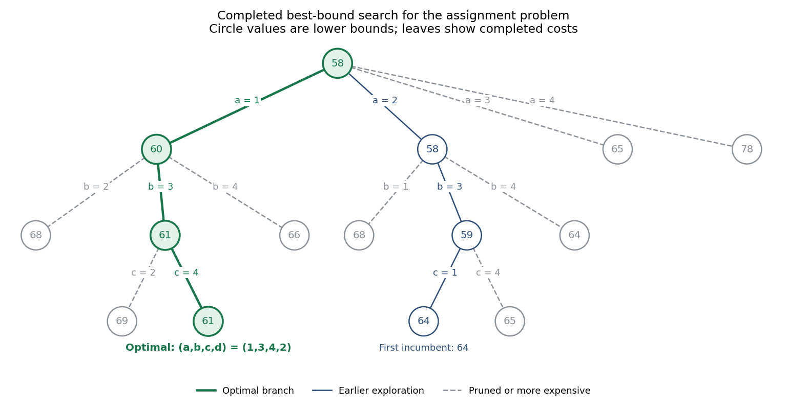
A branch and bound algorithm partitions the feasible set into subproblems and attaches a valid lower bound to each subproblem's possible objective value. A completed feasible solution supplies an incumbent upper bound. For minimization, discard a node if it is infeasible or its lower bound is at least the incumbent; otherwise branch by fixing an additional decision. The best-bound search rule expands the active node with the smallest lower bound. Once every active bound is at least the incumbent, the incumbent is optimal.
For this assignment problem, use the assignment lower bound from independent task minima. For a partial assignment , with unassigned machines and unassigned tasks , it isThis may reuse the same machine in several minima. Relaxing the distinct-machine constraint only reduces the cost, so the resulting lower bound is valid.
The given tree has already expanded the node of bound , then its child of bound . That child completes to at cost , or at cost . Thus we have an incumbent . The best remaining active node is , with lower bound . Its three branches have boundsThe first and third children cannot improve the incumbent. Expand , the sole active bound below . Its last two possible completions areUpdate the incumbent to . The unexpanded nodes have bounds , all at least ; the other completed leaves are also more expensive. The branch and bound search therefore terminates, withThe additional expansion order after the supplied tree is , then . The feasible assignment of cost and the bounds excluding every remaining branch together certify global optimality.


There are unlisted articles, also show them or only show them.