
In a finite additive group, a family of -subsets is a difference family of index one if each nonzero group element occurs exactly once among all their ordered within-block differences. Translating its Steiner blocks by every group element gives a Steiner system with parameters -: the unique representation of a difference determines the unique translated Steiner block through two specified points.
A designated subset in a Steiner system is a Steiner block. In a system , each Steiner block contains points and each -point subset belongs to exactly one Steiner block. For , this is the pair-coverage condition used in a cyclotomic construction of a Steiner 2-design.
Francis Galton used measurement of family resemblance to develop ideas that became central to regression and correlation. In his stature study, he grouped offspring heights by adjusted parental height and found that average offspring deviations were smaller than parental deviations. The Galton's stature regression article reconstructs his grouped data and the approximately two-thirds slope. This is a motivating example of regression toward the mean, rather than a law that every child must be closer to the population mean.[ref]
Regression towards mediocrity in hereditary stature by Francis Galton. 1886, printed pp. 247–248 and Plate IX(a), grouped family-height data and regression
His statistical programme was also bound up with advocacy of eugenics. UCL's institutional history documents the racial and social hierarchies behind that programme and the endowment that helped establish its early statistics department. That history belongs alongside his mathematical contributions.[ref]
https://www.ucl.ac.uk/mathematical-physical-sciences/statistics/about-us/our-history. UCL Statistical Science, Our History, Francis Galton and the early department

Portrait of Francis Galton
. Unknown photographer; Wellcome Library, London (institutional credit). CC BY 4.0, via Wikimedia Commons. Source.
In a location-scale family, for a fixed base probability distribution of , with and . Location translates observations, and scale multiplies their deviations. For an independent sample with a base density and at least two observations, the normalized residual vector , where , is an ancillary statistic. Indeed, and , making the residual vector a function of the base sample alone. This algebraic result needs no population moments.
A statistical model indexed by a parameter vector of fixed finite dimension is parametric. Examples include a normal distribution with unknown mean and variance and a Poisson distribution with unknown mean. Its likelihood function is the joint sample density or mass function, regarded as a function of the parameter at the observed sample.
A group action on the sample space induces a compatible action on the parameter space, preserving the family of probability laws. In a transitive model every law arises by transforming a fixed reference law. A location-scale model is generated by , , with parameter action .
Given the currently infected set and susceptible set , define and . Conditionally independent new-infection indicators have likelihoodA nonnegative infection intensity requires ; an unrestricted normal distribution prior distribution for must therefore be restricted or replaced. With or and positive distances, the conditional posterior kernels are not generally conjugate normal probability densities. Metropolis–Hastings algorithm updates, optionally on with its Jacobian determinant, provide a direct sampling method.
Decision tree learning fits predictors by recursively partitioning input space. Leaves predict labels for classification or numerical values for regression; a regression tree is the numerical-response case.
In statistical learning theory, Stability measures how much a learned predictor or its loss changes when the training sample is perturbed. Uniform stability of a learning algorithm imposes a bound valid at every test example.
Heteroskedasticity-consistent standard errors use an estimated regression covariance that remains consistent when error variances vary across observations. For ordinary least squares, the basic sandwich estimate is . The resulting standard errors are square roots of its diagonal entries. This is a regression application of a sandwich covariance matrix.
A chi-squared test rejects a null hypothesis for a statistic whose null distribution is a chi-squared law, exactly or asymptotically. Pearson tests compare observed and expected counts; both goodness-of-fit and chi-squared tests of independence are instances.
In a regular one-parameter statistical model, equality in the Cramér-Rao lower bound for an unbiased estimator implies the score function . Integrating in the parameter on a regular connected interval gives , with and . Thus efficiency for every parameter value forces an exponential family structure, under the usual common-support and differentiation assumptions.
All evidence in observed data about a parameter is contained in its likelihood function; proportional likelihoods carry the same evidence. If a stopping rule contributes only a positive factor independent of the parameter to the complete observed-sample likelihood, that factor does not change likelihood-based inference. Recording only a coarsened part of the sample produces a different likelihood and is not covered by the same invariance claim.
The one-sample Kolmogorov-Smirnov test checks goodness of fit by comparing an empirical distribution function with a specified cumulative distribution function . Its Kolmogorov-Smirnov statistic is the largest vertical gap anywhere between the two curves. Every threshold asks the same concrete question: what proportion of the observations are at or below it, and what probability does the proposed probability distribution assign there? A large discrepancy supplies evidence against the null hypothesis.
For example, four stipulated observations compared with the uniform distribution on give . Just before , only two observations have been counted, so the empirical distribution function approaches , while approaches . The Kolmogorov-Smirnov statistic section calculates every jump-side gap. These are exact illustrative numbers, not experimental measurements or a claim of statistical significance.
The ordinary one-sample calibration assumes independent and identically distributed real observations and a simple hypothesis , with a continuous function fixed before inspecting these observations. All statistical parameters of must be specified.[ref] Under that null hypothesis, the probability integral transform gives with the uniform distribution on , retaining independence. Consequently the sampling distribution of depends on the sample size , but not on the particular continuous . This is the useful sense in which the calibration is distribution-free.
For the exponential distribution of rate one, for . Take for the four stipulated above. The probability integral transform changes the horizontal coordinates but preserves both the order statistics and their cumulative heights, so the same Kolmogorov-Smirnov statistic appears on both scales. More generally, for continuous , the jump-side formulas depend only on . Strict increase everywhere is unnecessary: intervals on which is constant have probability zero under the null hypothesis. This explains the invariance without assuming a strictly positive probability density function.
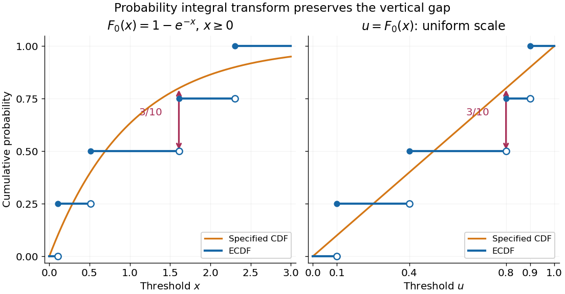
The probability integral transform preserves the Kolmogorov-Smirnov gap on exponential and uniform scales
. The same four stipulated points are shown as on the left and on the right. Open circles indicate left limits of the empirical distribution function, filled circles its values. The gap is approached from below the third observation on both scales. Details.
The observed Kolmogorov-Smirnov statistic is a discrepancy, whereas its p-value is a tail probability under the null hypothesis:Here is computed from a fresh sample of the same sample size. Choose a significance level before the test and reject when the calibrated p-value is at most . The value alone supplies neither a p-value nor a rejection decision. Failure to reject does not establish that the null hypothesis is true. A finite-sample calibration and the asymptotic Kolmogorov-Smirnov theorem are distinct; a cutoff for must be rescaled before use with .[ref]
Fitting statistical parameters on the tested observations replaces by the random . The resulting transformed observations need not be independent and identically distributed uniforms, so the ordinary reference law fails. The Lilliefors test addresses a particular fitted normal distribution. More general parametric bootstrap calibration must simulate from the fitted statistical model and repeat the fitting in every replicate; holding the fitted statistical parameters fixed during those comparisons calibrates a different procedure. Such a parametric bootstrap requires its own validity justification rather than inheriting exactness from the simple-null test.
For a discrete probability distribution, is generally not uniform. Equal observations also arise from rounding, so tied data require a calibration that accounts for the discrete probability distribution or the rounding rule. The discrepancy remains meaningful, but continuous-null p-values are not automatically valid. Statistical dependence likewise changes the reference law. The two-sample Kolmogorov-Smirnov test compares two empirical distribution functions and has a different calibration.[ref]
In a parametric statistical model, the likelihood function compares parameter values, while sampling distributions calibrate tests and confidence intervals. A sufficient statistic retains the parameter information. Conditioning on an observed ancillary statistic restricts that calibration to experiments with the same ancillary configuration, instead of averaging over configurations whose distribution is unrelated to the parameter. Since the ancillary's marginal law is parameter-free, conditional and unconditional likelihoods have the same parameter-dependent factor. With a nuisance parameter, a conditional law or pivotal quantity must remove it before inference for the parameter of interest can use a nuisance-free reference law.
The delete-one form of jackknife resampling recalculates a statistic after deleting each observation in turn. It uses one observed statistical sample to investigate how sensitive an estimator is to its individual observations, and supplies both a jackknife variance estimator and jackknife bias correction. The calculations are deterministic once the data are fixed: no random draws are needed.
In the basic setting, are independent and identically distributed random variables, with sample size . Let be the observed values and a scalar estimator of an estimand . Apply the same estimation rule to each reduced statistical sample, using its new sample size wherever the rule requires it:Every index is deleted exactly once; an unusual value is treated by the same rule as every other value. The mean summarizes the deletion estimates. They overlap in observations, so they are generally not independent random variables representing fresh repetitions of the original experiment. Cosma Shalizi's [ref]
https://stat.cmu.edu/~cshalizi/490/23/2023-11-29-jackknife.pdf. Carnegie Mellon jackknife notes, Sections 1–3 and 5
explain this construction and its scaling.For a concrete sample mean, use the data , whose full sample mean is . The five deletion sample means, in observation order, areDeleting raises the sample mean by , while deleting lowers the sample mean by . Thus has the largest deletion effect in this statistical sample. This is a descriptive sensitivity calculation, not a rule for removing that observation: the full sample mean remains .
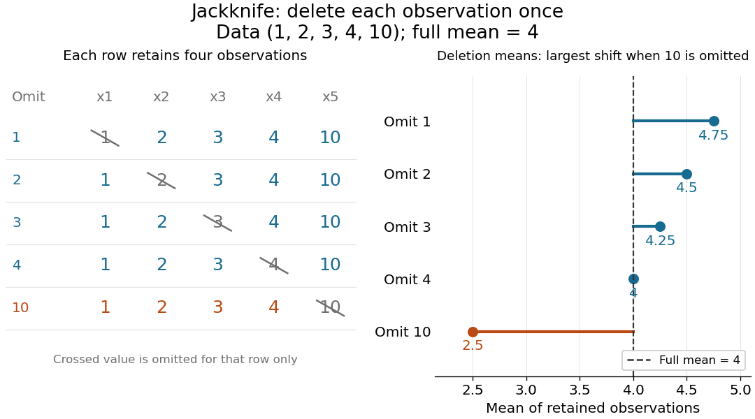
Delete each observation once and recompute the sample mean
. The left panel shows all five reduced statistical samples from ; each crossed entry is omitted only for that row. The right panel shows their sample means against the full sample mean . The orange row makes the deletion effect of visible. Details.
Early literature includes M. H. Quenouille's [ref]
https://academic.oup.com/jrsssb/article/11/1/68/7026551. Approximate Tests of Correlation in Time-Series, JRSS B 11(1), 68–84 (1949)
and John W. Tukey's one-paragraph abstract [ref]https://www.jstor.org/stable/2237363. Bias and Confidence in Not-Quite Large Samples, Annals of Mathematical Statistics 29(2), 614 (1958)
, within the issue's collected abstracts. Shalizi's [ref]https://stat.cmu.edu/~cshalizi/490/23/2023-11-29-jackknife.pdf. historical notes and bibliography
discuss the later development of jackknife bias correction and the jackknife variance estimator.Statistical process control compares observed process outcomes with a stable reference model and control limits reflecting expected sampling variation. An observation outside those limits is a signal to investigate, not proof of a specific cause. Varying sample volumes require varying limits, and multiple testing changes the chance of a chance signal somewhere in the display.
An effect size measures the magnitude of an observed or modeled relationship. A standardized mean difference expresses a mean contrast in standard-deviation units; other effect sizes include a correlation coefficient or odds ratio. Magnitude is distinct from the evidence against a null hypothesis supplied by a p-value: a small effect size can have a small p-value in a sufficiently large sample.
The pressure obtained by bringing a flow to rest without losses; in compressible flow the usual definition specifies an isentropic process for stopping. For the constant-mass density, same-height Bernoulli equation discussed under dynamic pressure, .
There are unlisted articles, also show them or only show them.