
Choosing a resident memory page to evict when another memory page needs an occupied page frame. An unused page frame needs no eviction. A dirty memory page requires preservation before reuse, accounted for separately as page writeback. A page replacement policy balances likely future reuse against the overhead of tracking past memory references.
The opportunity comes from temporal locality: retaining a recently accessed memory page can spare a later nonresident page fault. Spatial locality helps consecutive accesses reuse the same memory page until they cross its boundary. A working set describes recent demand, while the resident set describes what is actually present. A small active footprint can fit in the available page frames even when the whole address space cannot. These are useful workload tendencies, not guarantees about future memory references.[ref]
The page-reference trace below uses the counterexample discussed in Operating Systems: Three Easy Pieces by Remzi H. Arpaci-Dusseau and others (chapter 22, p. 5) and makes the decisions explicit. FIFO page replacement ranks arrival time, LRU replacement ranks last access, CLOCK page replacement samples recent use, and optimal page replacement knows the remaining sequence in advance. Count misses first; page-replacement cost accounting separately counts page writeback and explains why fewer misses need not mean less total service time.
// Destination: computer-science.bigb
Making a memory page resident when it is first accessed, using a page fault to request the work. It can involve loading stored contents or allocating newly initialized contents.
// Target: computer-science.bigb
A slot in main computer memory that can hold one memory page of the selected size. Physical frame number
0x07 with 256-byte page frames starts at physical address 0x0700.A contiguous unit of an address space used for paging. In the example, virtual page
0x12 consists of virtual addresses 0x1200 through 0x12ff.For a nonnegative integer and a prime number , the Legendre formula computes the prime exponent in a factorial without forming that huge product:Here is the floor function. The sum is finite: every term with is zero. When , all terms vanish, agreeing with and . The prime number hypothesis matters: a composite number does not give the same p-adic valuation or additive prime exponent. For example, the floor sum with is one, whereas divides .
Why count multiples repeatedly? Each multiple of in contributes one factor of ; each multiple of contributes another; and so on. A factor with p-adic valuation occurs in exactly the first counts. Adding those contributions proves the formula.[ref]
Number Theory for Mathematical Contests by David Anthony Santos. David A. Santos, Number Theory for Mathematical Contests, revision 31 October 2007, §8.3, Theorem 245, printed pp. 89–90: factorial valuation and digit form
For the original example ,The five multiples each contribute a second factor of three. The factor contributes a third, so it appears in all three rows. Equivalently, among there are eleven factors of p-adic valuation one, four of valuation two, and one of valuation three: . Thus divides , while does not.
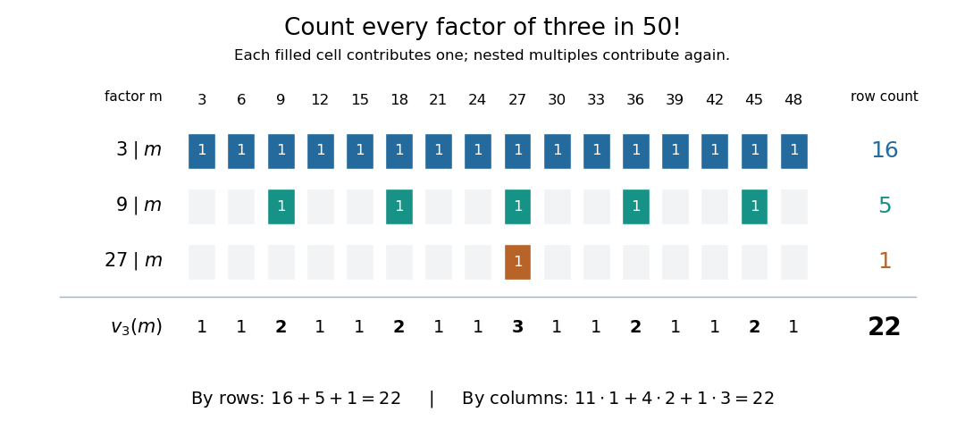
Nested multiples count the factors of three in
. Each colored cell contributes one to the p-adic valuation. Multiples of nine occur in two rows, and occurs in three. Summing by rows gives ; summing by columns gives . Factors not divisible by three contribute zero and are omitted. Details.
Repeated Euclidean division provides a practical evaluation: replace by , starting from , and add each new quotient until it is zero. This uses only the successive quotients for the example. The same calculation handles divisibility of binomial coefficients, where the p-adic valuations of the denominator factorials are subtracted.
Oxygen-16 is the stable oxygen isotope with eight protons and eight neutrons. It is the most abundant oxygen isotope in ordinary terrestrial material.
Its nucleus has spin zero, unlike oxygen-17, so isotope choice changes which nuclear-magnetic-resonance experiments are possible. Isotopic identity therefore affects both mass-sensitive measurements and nuclear-spin observability without changing the element's proton number.
An oxidation state is an electron-bookkeeping assignment to a chemical atom: its electric charge number after the ionic approximation of bonds. It helps identify oxidation and reduction and determine stoichiometry, even for covalent bonds without separate charged ions. In water, each hydrogen has oxidation state and oxygen has ; this does not assert that a water molecule contains two free protons and a free oxide ion.[ref]
Comprehensive definition of oxidation state (IUPAC Recommendations 2016) by Pavel Karen and others. Karen, McArdle and Takats, Comprehensive definition of oxidation state (IUPAC Recommendations 2016), §2, pp. 832–833: definition and equal splitting of same-element bonds
Three conventions answer different questions. Formal charge divides each bonding electron pair equally in a chosen Lewis structure. Oxidation state uses the ionic approximation of bonds. Partial atomic charge instead partitions the actual electron density and depends on that partition. In the ordinary water Lewis structure, every formal charge is zero although the oxidation states are not. Neither bookkeeping convention supplies numerical partial atomic charges.
An upward angular spectrum obtained from a horizontal field trace is exact in the homogeneous half-space above that reference plane. For a rough boundary , choose the plane above . A trace at is not physically defined in the medium if any part of the surface lies above it. Using such a mean-plane trace requires an analytic continuation convention; convergence of the continued spectrum down to the rough boundary is an additional hypothesis. Small-height boundary perturbation uses the reference plane formally order by order and is distinct from an exact expansion throughout an arbitrary rough domain.
Use and on the upward branch. If the uncentered field correlation is translationally homogeneous and , its correlation at height is the displayed integral. The propagating spectrum is unchanged; evanescent contributions decrease as . A spectral measure of a stationary random field permits discrete coherent components. Without correlation homogeneity a double spectral covariance integral depends on both observation coordinates rather than only their separation.
Correlation-based learning among spatially arranged ON and OFF inputs, with synaptic competition and lateral interactions, can select elongated simple cell receptive fields. Neighbor interactions coordinate preferred orientations across cortex, while competition allows different orientations to persist. Selectivity within one cell and a spatial map across many cells are separate predictions, and neither follows from unbounded Hebbian learning alone.
An orientation tuning curve plots a specified response against the stimulus-axis angle , with the other stimulus variables controlled. A practical count summary for extracellular single-unit recording iswhere counts action potentials in the same duration on trial , and is the number of repeats at each angle. This estimates spikes per unit time in that window; the window must specify whether it covers onset, sustained stimulation, or both. Record a blank-background response separately, and report whether it has been subtracted. Randomizing angle order and repeating each condition helps separate orientation selectivity from changes over time, including neural adaptation. This is a proposed measurement procedure, not a claim that the original experiments used this estimator.
A simple cell's orientation tuning curve can also change when the stimulus shifts. An angle sweep at fixed phase, a sweep averaging over phase, and a sweep of moving stripes ask different questions. Consequently, a single preferred angle does not specify the whole receptive field. The toy curve under orientation selectivity holds phase fixed and plots dimensionless output, rather than spikes per second.
For a differentiable radial factor and integer , the coordinate polynomial obeys and . The identity gives the displayed angular eigenvalue. Lowering gives , a nonzero eigenfunction with the same angular eigenvalue when and the original state is nonzero. At lowering gives the zero function, which is not an eigenfunction. Negative powers satisfy local differential identities off the axis but are not regular angular states.
The orbifold fundamental group is the group of deck transformations of the universal orbifold cover. It retains the local finite group data that the ordinary fundamental group of the underlying topological space forgets.[ref]
The Geometry and Topology of Three-Manifolds by William Thurston. Chapter 13, Definition 13.2.5, page 307
For an oriented closed topological surface of genus with cone points of orders , the group presentation isEach local cone relation says ; it does not guarantee that has order exactly in the resulting global group. For the teardrop orbifold, a two-sphere with one cone point of order , the remaining relation is , so its orbifold fundamental group is trivial despite nontrivial local isotropy.[ref]
The Geometry and Topology of Three-Manifolds by William Thurston. Chapter 13, Definition 13.2.3 and the teardrop example, page 304
For a complete hyperbolic surface orbifold, the universal cover is the hyperbolic plane. A torsion-free finite-index subgroup then acts freely and gives a smooth surface cover. The hyperbolic covering model is what identifies local cone stabilizers with actual finite subgroups in this case.
For wealth dynamics and utility , with and , the unconstrained interior control equations do not give the maximum. Put . At positive shadow price , maximization over leaves a function of proportional to , up to constants. It is convex and hence maximal at or . The optimal controls work with zero consumption first, then cease work and consume at . The switch occurs where this consumption reaches ; the full discounted budget fixes and the switch time. The decreasing-consumption interior stationary candidate violates the Hamiltonian maximization condition.
Quantum optimal control minimizes a state-transfer, observable, or gate error together with resource costs, subject to a controlled Schrödinger equation or Lindblad equation. Forward propagation of the state and backward propagation of a costate compute the gradient efficiently. The optimum depends on the admissible time-dependent fields and laboratory constraints.
For and with independent unit-variance normal noises, the equilibrium prediction-error variance is . Orthogonality to the next innovation gives the filtering gain . Minimizing the quadratic average cost gives a control Riccati coefficient satisfying , so and . Completing the control square yields minimal cost . The one-step observation delay is essential to the value of .
For bank dynamics and utility , substituting the terminal balance separates the concave optimization pointwise and gives the displayed control for . Put and . Its terminal balance is , so the unique positive multiplier achieving zero terminal wealth is . The same control solves the problem with no terminal reward and constraint , by the supporting-line inequality for logarithms.
An optical momentum efficiency expresses the net axial momentum transferred to a bead relative to incident power divided by vacuum light speed. It absorbs medium-index factors and the incident/outgoing ray geometry. Refractive-index contrast alone does not determine for a transparent bead illuminated by a focused beam. The estimate is a weak-contrast scale, not a universal force formula. An effective reflector with power reflectance instead gives in the simple vacuum-momentum convention.
A harmonic optical trap approximates one coordinate near a stable equilibrium by a quadratic potential energy. Measure displacement from that equilibrium, set its potential energy to zero there, and take a positive effective spring constant , also called the trap stiffness:The restoring force points left when and right when . This is a local model: a Taylor series of a smooth potential energy about a nondegenerate local minimum gives as its leading curvature. A real optical trap has a finite capture region; the endlessly rising parabola does not describe its escape boundary. A three-dimensional optical trap can have different stiffnesses along different axes, and nonconservative optical forces can limit the potential energy description.
An optical scattering force transfers momentum from light to a particle through scattering of light. In a usual single-beam optical trap, its axial contribution pushes along beam propagation; the optical gradient force must balance it for axial confinement. This balance can place the stable equilibrium away from the beam focus.
There are unlisted articles, also show them or only show them.