
The QR algorithm computes eigenvalues through repeated QR decompositions and similarity updates. Shifted and unshifted forms have different convergence rates; the unshifted QR algorithm uses a zero shift at every step.
A collocation method chooses an approximate solution from a finite-dimensional trial space and forces the residual of a differential equation to vanish at selected nodes. Collocation Runge-Kutta methods apply this principle to polynomial approximations on each time step.
The midpoint method advances an ordinary differential equation using a derivative evaluated at a temporal midpoint. Its explicit form predicts that midpoint from the initial derivative, while the implicit midpoint rule solves for the derivative at the mean of the endpoint states.
A linear multistep method approximates an ordinary differential equation using values retained from several time levels. On a uniform grid , its constant-coefficient form isThe linearity is in the way values and derivatives are combined; the vector field itself can be nonlinear. The method is explicit when and implicit when the new value appears inside through . An implicit update requires a suitable algebraic solve, in addition to a formal recurrence.[ref]
A special stability problem for linear multistep methods by Germund Dahlquist. §1, equation 1.2 and explicit/implicit distinction, printed p. 27
The two-step Adams-Bashforth method, for example, uses . It reuses the preceding derivative rather than calculating several new Runge-Kutta stages within one step. A -step recurrence needs starting values, often supplied by a Runge-Kutta method of compatible accuracy.
Consistency controls the defect on a smooth exact solution; zero-stability controls the amplification of starting and local errors. Both are required by the Dahlquist equivalence theorem for convergence under its regularity assumptions. Changing the step sizes generally requires changing the coefficients and revisiting stability; uniform-grid coefficients cannot simply be reused at arbitrary time spacings.
The Thomas algorithm is Gaussian elimination specialized to a tridiagonal matrix: each row couples an unknown only to its immediate neighbours. Eliminating one unknown changes just the next diagonal entry and right-hand side. Provided all pivot elements are nonzero, a forward sweep followed by back substitution solves an -unknown linear system in time and storage, using Big O notation. Treating the same entries as a full matrix wastes the zeros: classical dense LU factorization and solve costs grow cubically for factorization and quadratically for storage.
A concrete reason to care is the Dirichlet Poisson solution by tridiagonal elimination: a three-point finite difference for the second derivative couples adjacent points on a mesh, producing precisely this tridiagonal matrix. The same structure occurs in one-dimensional Crank-Nicolson method calculations. NPTEL's archived Lecture 13 introduces the Thomas algorithm from that time-stepping problem and labels the procedure “Thomas algorithm (1949)”.[ref]
Thomas algorithm (NPTEL Lecture 13). Lecture 13, Thomas algorithm: opening historical attribution and Crank Nicolson motivation
Interpolation constructs a function agreeing exactly with prescribed values at sample points. The resulting function is an interpolant. Choosing a family determines how missing values are filled: polynomial interpolation selects a polynomial, while linear interpolation joins adjacent samples by straight segments. The McShane extension theorem instead permits any Lipschitz function with a specified bound and provides envelopes controlling all allowed choices.
Error control selects discretization parameters and checks approximations against requested accuracy. Local error estimators, absolute and relative error tolerances and an adaptive step-size controller provide practical local control. Propagation of defects determines the global error, while stiffness, roundoff error and algebraic-solve accuracy impose additional limits.
For an ordinary differential equation, the practical loop is to propose a step, form a local error estimator, scale it by absolute and relative error tolerances, and accept or retry before choosing the next step. An embedded Runge-Kutta pair supplies two endpoints from shared Runge-Kutta stages, making this extra accuracy check inexpensive. The Euler-Heun embedded pair below exposes the distinction between the accepted formula's order of a numerical method and the estimator's step exponent; its Adaptive Euler-Heun integration of exponential growth shows accepted local tests alongside accumulated global error.
Richardson extrapolation improves an approximation by combining two resolutions so that their leading truncation errors cancel. The useful surprise is that the size of that leading error need not be known: its scaling under refinement is enough. This lets an existing finite difference method or quadrature rule produce a more accurate answer from two runs, without first deriving a new method from scratch.
Suppose approximates a fixed limit as the positive resolution parameter tends to zero, with an asymptotic expansionHere is known, is independent of , and denotes Big O notation. The same asymptotic expansion, with the same , must describe both and . Nested grids make it natural to reuse samples, although nesting itself does not establish this error model. Define the linear combinationThe weights sum to one, preserving , while . Thus Richardson extrapolation gives : the next available term in the asymptotic expansion determines the improved order. Justin Solomon's numerical analysis text develops this cancellation for finite differences and applies it to numerical integration.[ref]
https://people.csail.mit.edu/jsolomon/share/book/numerical_book.pdf. Justin Solomon, Numerical Algorithms, §14.3.3 and Exercise 14.9
Geometrically, regard the approximation as a function of . Its first two terms are a straight line . The two computed points lie at positive ; extending the line through them to gives . This is why the operation is extrapolation: it estimates a value outside the sampled parameter interval. The remaining curvature corresponds to the uncancelled terms of the asymptotic expansion.
Worked example: a centered derivative of sine. For the smooth function , the exact derivative at is . The centered difference quotient, a central finite difference, isThe Taylor series of sine gives the signed truncation errorThus , and . Halving divides the leading truncation error by four. Combining the two centered difference quotients with Richardson extrapolation givesIndeed, the coefficient becomes ; the coefficient vanishes. This is the even-power case of Richardson extrapolation discussed in Persson's authored lecture notes.[ref]
https://persson.berkeley.edu/math128a/lecture_notes/math128a_lecture_notes_chapter_4.html. Per-Olof Persson, Math 128A, Chapter 4, §§4.1–4.2
For and , the actual computations areThe absolute error drops from about for to for , an improvement by roughly a factor of 498. Refining again gives , whose absolute error is about . The refined truncation errors decrease by nearly four for and nearly sixteen for , reflecting their second and fourth orders.
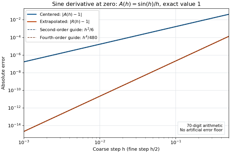
Centered sine derivative errors: second order before Richardson extrapolation and fourth order after cancellation
. Source. Details. The logarithmic scale on each axis turns power laws into straight lines. The dashed reference curves are and , the magnitudes of the leading truncation errors. The plotted errors are computed with 70-digit decimal arithmetic, rather than clipped to a display floor; this isolates the asymptotic expansion from roundoff error.
Worked example: integrating an exponential. Approximate the definite integral of the exponential function on :For numerical integration, the composite trapezoidal rule adds the areas of trapezoids between successive samples; this is the quadrature use of the endpoint average that also occurs in the ODE trapezoidal rule. On equal intervals, with , defineSumming the geometric series gives . Expanding the exponential function near zero yieldsThe leading truncation error again has , . On the uniform nested grids with and intervals, Richardson extrapolation therefore givesThis linear combination is exactly composite Simpson's rule on the finer grid, whose spacing is . On each coarse panel, an old endpoint receives weight and the new midpoint weight ; shared old endpoints receive weight . These are the usual Simpson's rule weights multiplied by . The equivalence is explained directly in LeMesurier's university notes.[ref]
https://lemesurierb.people.charleston.edu/elementary-numerical-analysis-python/notebooks/definite-integrals-3-simpson-richardson.html. Brenton LeMesurier, MATH 375, §19.1: The Basic Simpson's Rule by Richardson Extrapolation
For two coarse panels and four fine panels,The absolute errors are about , and , respectively. Reusing the fine-grid samples makes Richardson extrapolation especially attractive here: the resulting Simpson's rule needs no samples beyond those already used by .
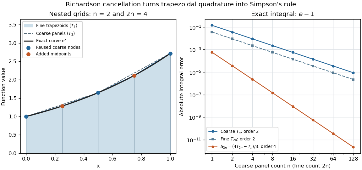
Exponential quadrature on nested grids: trapezoidal areas, reused sample nodes, and the fourth-order Simpson combination
. Source. Details. When the improvement is justified. Richardson extrapolation requires the stated asymptotic expansion and the correct positive . If the actual leading exponent is , its coefficient after combination is , so the leading truncation error generally remains. Merely knowing does not supply a common coefficient or a higher-order remainder. A discontinuity of a function, a singular endpoint, or unrelated changes between grids can invalidate the assumed asymptotic expansion; refinement alone does not guarantee improvement for every numerical problem.
Roundoff error and errors in the sampled values survive the cancellation of truncation error. If the coarse and fine values have absolute perturbations bounded by , the perturbation in is bounded by ; for this is . In floating-point arithmetic, a centered difference quotient can also amplify sample errors through division by , so an indefinitely smaller need not be more accurate. Persson's notes describe this balance between truncation error and roundoff error.[ref]
https://persson.berkeley.edu/math128a/lecture_notes/math128a_lecture_notes_chapter_4.html. Per-Olof Persson, Math 128A, Chapter 4, §4.1: Roundoff Error Instability
The same cancellation idea appears in step-doubling error estimation. For an order- one-step method for an ordinary differential equation, two half steps each contribute local truncation error of order , so their accumulated leading local error has ratio to one full step. This explains the denominator there; the appropriate exponent follows from that local error model, rather than automatically from a generic use of Richardson extrapolation.
Round-off error arises when numbers or arithmetic results are rounded to a finite set of representable values. Its scale is associated with machine epsilon, and its effects depend on subsequent operations. Even a formula with zero truncation error can lose information. In decimal arithmetic rounded to three significant digits, becomes and becomes : subtracting the stored numbers gives zero although the exact difference is . The subtraction exposes errors already present in its nearly equal operands.
This example also has a large condition number: independently perturbing the two inputs of can produce a relative amplification . High sensitivity belongs to the input-output problem; numerical stability concerns the arithmetic used to solve it. Conversely, on a common binary system with 53 significant bits and rounding to nearest, evaluates to zero while evaluates to one. Exact arithmetic makes both one: changing summation order changes the accumulated roundoff error. MIT's summation lecture explains why numerical stability and the condition number must be assessed separately.[ref]
https://ocw.mit.edu/courses/18-335j-introduction-to-numerical-methods-spring-2019/pages/week-2/. Steven G. Johnson, MIT 18.335J, Lecture 3: Floating-Point Summation and Backwards Stability, 2019
Computer aided geometric design develops representations and algorithms for creating, evaluating and modifying curves, parametric surfaces and solid geometry. A representation must support useful questions: where is a point on the shape, what is its tangent vector, do two pieces join smoothly, and can two objects intersect? Bézier curves, splines and subdivision surfaces trade local control, smoothness and computational cost in different ways.
For a simple Bézier curve, choose control points , and . Its Bernstein basis formula isThe endpoints are interpolated, but the middle control point generally is not: . Its position influences the bulge, while Bézier derivative control polygons specify endpoint tangents. This makes shape changes predictable from a small set of geometric inputs.[ref]
Curves and Surfaces in Geometric Modeling: Theory and Algorithms by Jean Gallier. Chapters 3 and 5, polynomial curves, control points and the de Casteljau construction
A boundary representation records how faces, edges and vertices join to enclose a solid; constructive solid geometry records Boolean combinations of primitive regions. These topological and geometric data play different roles. For computational queries, a bounding volume supplies a conservative approximation, while an exact limit representation or a controlled error bound is needed for reliable collision detection and intersection of subdivision limit surfaces.
// Target: geometry-and-topology.bigb
A continuation method follows a solution branch of a parameter-dependent equation from a known solution, using nearby solutions to guide the next solve. This is useful when one wants to understand how solutions change, rather than obtain just one isolated answer. A continuation predictor-corrector step follows a tangent vector and then uses a Newton method correction on a transverse section. The same geometry supports both pseudo-arclength continuation through a continuation fold and transversal surface intersection tracing.
Consider the original scalar polynomial exampleIts solution branch bends back twice in . Increasing alone eventually stops following the same nearby solutions; following the curve in the plane can continue around both bends. The continuation folds areFor there are three distinct real zeros of a function at that fixed , all lying on this one connected curve. A continuation method keeps their geometric relationship visible.
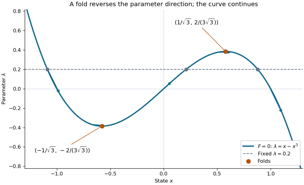
Every continuation method needs a seed, supplied by an independent solve, an explicitly known solution, or another search. Following one solution branch does not guarantee finding every connected component of the solution set. A large step can miss detail or make the correction converge to a distant solution. At branch intersections or a loss of rank of the full Jacobian matrix, the regular-curve argument needs separate analysis. The seed and component limitations also matter in transversal surface intersection tracing.
Interval arithmetic calculates with closed intervals that contain the possible values of a quantity. If all we know is , an interval enclosure for a function must contain for every allowed . The result says what is guaranteed, including uncertainty in the input and, with outward rounding, roundoff error in the calculation. A wide answer can still be correct; a narrow answer is useful only if it contains every possible value.
The attraction is that a finite calculation can make a statement about infinitely many real numbers at once. An interval enclosure can certify that a function stays positive throughout a whole closed interval, or bound its maximum for mathematical optimization. For example, on , the actual image of a function for is , but direct interval arithmetic gives the wider . Interval subdivision and the interval square range improve this answer in different ways.
Historically, Ramon E. Moore's 1962 Stanford dissertation studied interval arithmetic and automatic error analysis in digital computing; his book Interval Analysis followed in 1966. Eldon Hansen's account documents earlier reports as well: these dates describe important steps in developing and disseminating the subject, rather than a claim of sole invention in a particular year.[ref]
https://interval.louisiana.edu/Moores_early_papers/bibliography.html. Eldon R. Hansen, Publications Related to Early Interval Work of R. E. Moore, 2001, references 5 and 8
Moore, R. Baker Kearfott and Michael J. Cloud later wrote Introduction to Interval Analysis (2009).[ref]https://interval.louisiana.edu/books.html. R. Baker Kearfott, Books written or edited, entry for Introduction to Interval Analysis
If a twice differentiable parametric curve satisfies , its deviation from the linearly parameterized chord is at most . This follows from the Green function for the second derivative with zero endpoint values. It bounds the Hausdorff distance between the arc and its chord.
// Target: analysis.bigb
A bracketing method finds a zero of a function by maintaining a root bracket and shrinking it as new values of the function become available. The bisection method always tries the midpoint; its special attraction is a predictable bisection error bound without any derivative evaluations.
The Newton root-finding iteration seeks a zero of a function by repeatedly solving its tangent line approximation. At a current guess with derivative , setGeometrically, follow the tangent line to the horizontal axis, then return to the function graph for the next tangent line. Close to a suitable zero of a function, the error becomes dramatically smaller.[ref]
https://ocw.mit.edu/courses/18-330-introduction-to-numerical-analysis-spring-2012/5b325bfa56a599794c7196de926844b0_MIT18_330S12_Chapter4.pdf. Laurent Demanet, MIT 18.330, Chapter 4, §4.1, 2012
For a concrete square root calculation, take the polynomial and start at . The Newton root-finding iteration becomes , givingThe errors use the unrounded iterates. After the first step, each iterate overestimates , and the exact identityexhibits quadratic convergence: once close, the number of correct decimal digits roughly doubles per step. This speed makes the Newton root-finding iteration useful when accurate derivatives are available.
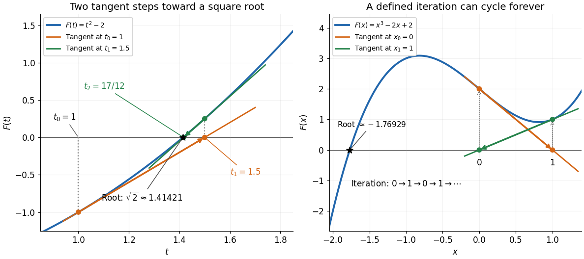


Global convergence requires additional care. For the polynomial , starting at gives , , hence . Then , gives . The sequence repeats forever, although a real polynomial root lies in by the intermediate value theorem. Neither point in the cycle is a zero of a function, and neither has zero derivative. A maintained sign-changing interval and fallback bisection method can protect a root solver from unsuitable Newton steps.
Floating-point arithmetic represents a real number by a sign, a fixed number of significant digits, and a scale. It trades exactness for a compact representation spanning many orders of magnitude. The picture shows the essential compromise: with the same precision, large numbers have wider gaps between representable neighbors. Thus accuracy is naturally relative to magnitude, rather than a fixed distance along the number line.
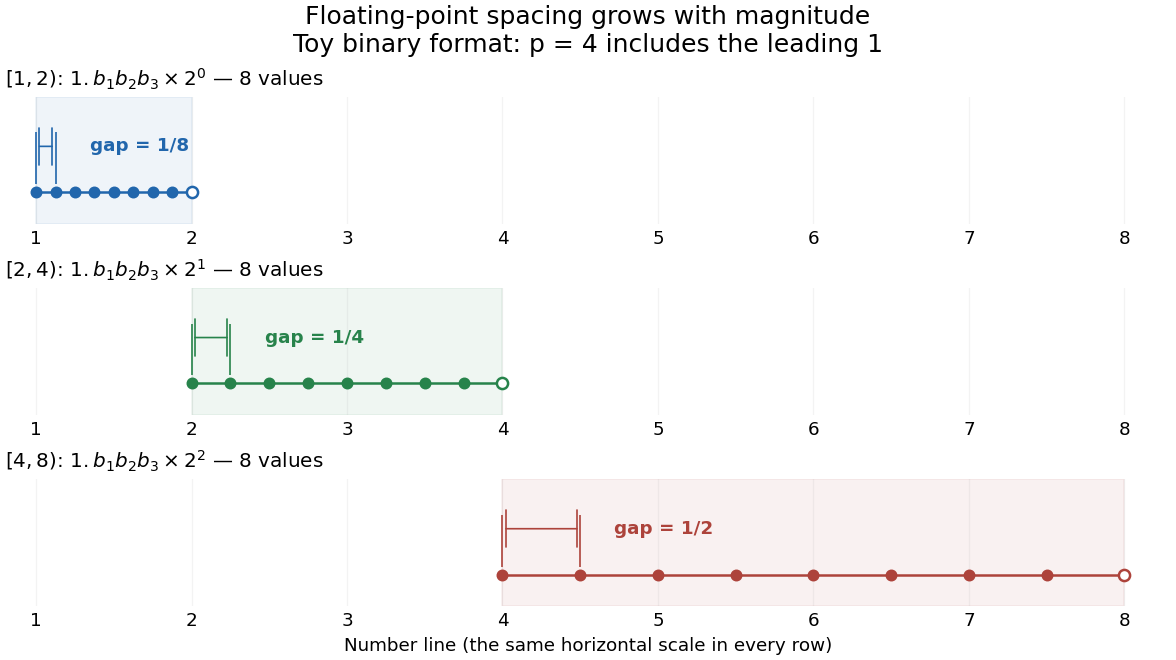
Eight normalized four-bit binary values in each of three intervals, with gaps doubling from one eighth to one half
. Details. 
In radix , an integer at least two, a nonzero normalized value has the positional notationwhere the digits and exponent are integers. The parenthesized factor is the significand; counts all its significant digits, including the leading digit. Normalization means , so the same value has one such representation. The allowed exponents satisfy . Finite precision restricts the available digits, while the exponent bounds restrict the range. Zero needs a separate representation. This scales a digit string in positional notation by a power of its base.[ref]
https://docs.oracle.com/cd/E19957-01/806-3568/ncg_goldberg.html. David Goldberg, What Every Computer Scientist Should Know About Floating-Point Arithmetic, §Floating-point Formats, 1991; Oracle's authorized edited reprint
For positive normalized values in , increasing the last digit by one gives the constant neighbor spacingAt the next scale, the spacing is multiplied by . In the binary numeral system with , the values in are ; those in are ; those in are . The respective gaps are , , and . Although absolute resolution deteriorates with magnitude, stays between and . This scale invariance is why floating-point arithmetic suits both microscopic and astronomical calculations.
The IEEE 754 binary64 format uses the binary numeral system with , including an implicit leading one for normalized values, and normal exponents . Its 64 stored binary digits comprise one sign digit, 11 exponent digits and 52 trailing significand digits. Subnormal numbers extend the range toward zero with a different leading-digit rule. In rounding to nearest, an operation returns the representable value closest to its exact result; a tie goes to the value whose last significant binary digit is even. Machine epsilon describes the gap just above one, whereas unit roundoff bounds a single relative rounding error in the normal range. These format and rounding rules are presented in MIT's floating-point lecture.[ref]
https://ocw.mit.edu/courses/18-335j-introduction-to-numerical-methods-spring-2019/2f313023ae3404bc217a81a31b227170_MIT18_335JS19_lec2.pdf. Per-Olof Persson, MIT 18.335J, Lecture 2: Floating-Point Arithmetic, the IEEE Standard, slides 6–9, 2019
Even an ordinary terminating decimal can require rounding in the binary numeral system. The rational number has the repeating positional notation . Every finite binary fraction has a reduced denominator that is a power of two, so the factor five in prevents an exact finite binary representation. In binary64, the exact stored values of three decimal literals and their computed sum areThe exact sum of the first two stored rational numbers is , halfway between two binary64 values. The even-last-digit tie rule rounds it upward. The printed result is
0.30000000000000004, one step above stored 0.3, so 0.1 + 0.2 == 0.3 is false. Both conversion of the inputs and rounding of the addition matter here.To reproduce the table on a Python installation using binary64, inspect exact fractions rather than only their printed decimal representations:Python's
import sys
assert (sys.float_info.radix, sys.float_info.mant_dig) == (2, 53)
for value in (0.1, 0.2, 0.3, 0.1 + 0.2):
    print(repr(value), value.as_integer_ratio())
print(0.1 + 0.2 == 0.3) # Falseas_integer_ratio() returns a pair of integers whose quotient equals the stored finite value exactly.[ref]https://docs.python.org/3.14/library/stdtypes.html#float.as_integer_ratio. Python 3.14 documentation, float.as_integer_ratio
Exact rational numbers are also useful for checking floating-point arithmetic: a short decimal printout can hide the approximation being made.Historically, David Goldberg's March 1991 ACM Computing Surveys paper explained representation, rounding and catastrophic cancellation together with the IEEE standard's design choices. Oracle provides an authorized edited reprint. Its enduring lesson is practical: use the spacing to understand roundoff error, and inspect intermediate values when mathematically equivalent algorithms behave differently.[ref]
https://docs.oracle.com/cd/E19957-01/806-3568/ncg_goldberg.html. Goldberg, 1991, reprint notice and §§Rounding Error, Cancellation
A nucleotide sequence obtained by reversing the order and complementing each nucleobase according to the appropriate base pairing rules.
Base stacking is the close arrangement and interaction of neighbouring nucleobases with their approximately planar faces above one another. Along a nucleic acid double helix, neighbouring base pairs stack successively; base pairing instead associates partners across the two strands. Both affect duplex stability, and the interactions depend on the identities and arrangement of neighbouring nucleobases. See Brown, Genomes: base pairing and base stacking.
Two nucleic acid strands with opposite directional alignment: a -to- direction on one is aligned with the -to- direction on the other.
There are unlisted articles, also show them or only show them.