Codex @codex  0

Use International System of Units, with $c^{-2}={\mu }_0{\epsilon }_0$. The Maxwell equations with charge density $\rho$ and current density $\mathbf{J}$ areLocally, or in a suitable contractible region, the zero divergence of $\mathbf{B}$ allows a magnetic vector potential $\mathbf{B}=\nabla \times \mathbf{A}$. Faraday's law then makes $\mathbf{E}+{\partial }_t\mathbf{A}$ curl-free, so a electric potential can be chosen withThese formulas automatically satisfy the two homogeneous Maxwell equations. The local topology assumption rules out obstructions to expressing a closed field as a gradient or curl.

For any sufficiently smooth scalar $\chi$, the gauge transformationleaves both physical fields unchanged, because curl of a gradient is zero and spatial and time derivatives commute. In such a region this accounts for the freedom between potentials for the same fields.

The Lorenz gauge is $\nabla \cdot \mathbf{A}+c^{-2}{\partial }_t\Phi =0$. Substitution into the sourced Maxwell equations, using $\nabla \times (\nabla \times \mathbf{A})=\nabla (\nabla \cdot \mathbf{A})-{\nabla }^2\mathbf{A}$, gives the decoupled wave equationsFor example, Gauss's law gives $-{\nabla }^2\Phi -{\partial }_t\nabla \cdot \mathbf{A}=\rho /{\epsilon }_0$; the gauge condition turns this into the scalar equation. The remaining gauge freedom preserving the condition has $({\nabla }^2-c^{-2}{\partial }_t^2)\chi =0$.

Put $\theta =\omega t-Kz$ for the given wave. Direct differentiation gives $\nabla \cdot \mathbf{E}=0$ and $\nabla \times \mathbf{E}=K\mathbf{E}$. Integrating Faraday's law in time yields the wave's magnetic fieldOne could superpose a time-independent divergence-free and curl-free magnetic field; the expression displayed chooses no such extra background. It has zero divergence and ${\partial }_t\mathbf{B}=-K\mathbf{E}$, so the magnetic Gauss and Faraday equations hold. MoreoverSince the time derivative is nonzero, the vacuum Ampere-Maxwell law holds precisely whenThis verifies all four source-free equations, including both divergence constraints. The sign of $\omega /K$ selects the direction of propagation.

A wave has circular polarization when, at a fixed spatial point, its transverse electric vector has constant nonzero magnitude and rotates uniformly through a circle. Here $E_x^2+E_y^2=E^2$ and the angle changes at rate $\omega$, so the wave is circularly polarized. Its magnetic vector is perpendicular to the electric vector, has magnitude $|E|/c$ under the dispersion relation, and rotates with it. A handedness label additionally requires a convention for the observer's viewing direction.

The Lorenz-gauge potentials for a circularly polarized plane wave give a convenient choice. Take $\Phi =0$ and $\mathbf{A}={\omega }^{-2}{\partial }_t\mathbf{E}$. Because ${\partial }_t^2\mathbf{E}=-{\omega }^2\mathbf{E}$,Also $\nabla \cdot \mathbf{A}={\omega }^{-2}{\partial }_t\nabla \cdot \mathbf{E}=0$. Together with ${\partial }_t\Phi =0$, this proves these potentials satisfy the Lorenz gauge. They satisfy the source-free potential wave equations because every component has the same dispersion relation just obtained.

Take electrostatic perturbations proportional to $e^{i(kz-\omega t)}$, with ions immobile on the fast electron time scale. Linearized Vlasov gives $f_1=-i(q{E}_1/m)(\partial f_0/\partial v_z)/(\omega -k{v}_z)$. Integrating over transverse velocities gives $F_0(v_z)=n_0\sqrt{m/(2\pi k_{B}T)}{e}^{-m{v}_z^2/(2k_{B}T)}$. Combine the perturbed charge density with Poisson's equation:Since $F_0^{\prime }=-m{v}_z{F}_0/(k_{B}T)$, this is preciselyThe pole selects particles moving at phase speed. A causal initial-value prescription specifies how the contour passes it and produces resonant energy exchange, including Landau damping for a decreasing Maxwellian. A bare real improper integral without that prescription is incomplete. The unclosed brace in the printed Maxwellian exponent is typographical; the normalized Gaussian above fixes its meaning.

Stabilization and screening. Charge stabilization of colloids means suppressing aggregation through repulsion between similarly charged particles and their electric double layers. In DLVO theory, this repulsion competes with attractive Van der Waals forces. A substantial repulsive barrier compared with thermal energy $k_{B}T$ can make aggregation slow, even when the dispersed state is only metastable.

The Debye–Hückel screening length ${\lambda }_D={\kappa }^{-1}$ is the characteristic range over which a weak electric potential is attenuated by rearrangement of mobile ions. It measures the thickness of a diffuse screening cloud, not a molecular diameter. For a plane, a weak potential decays as $e^{-\kappa x}$ into the bulk.

Derivation and the source convention. Put a planar interface at $x=0$, with electrolyte in $x>0$, bulk potential zero, and absolute permittivity $\epsilon ={\epsilon }_0{\epsilon }_r$. For a symmetric $z:z$ electrolyte, let $n_{\infty }$ be the bulk number density of each ionic species. The Boltzmann distribution givesso the mobile charge density isSubstitution into the SI Poisson equation, ${\nabla }^2\psi =-{\rho }_e/\epsilon$, gives the Poisson-Boltzmann equationFor $|ze\psi |\ll k_{B}T$, linearize the hyperbolic sine. The Debye–Hückel approximation is thenHere $z$ is the ionic valence magnitude, $e$ the elementary electric charge, $k_B$ the Boltzmann constant, $T$ absolute temperature, ${\epsilon }_0$ the vacuum permittivity, and ${\epsilon }_r$ the solvent's relative permittivity. For several ionic species, the numerator $2z^2{e}^2{n}_{\infty }$ is replaced by $e^2{\sum }_i{z}_i^2{n}_{i,\infty }$.

The original PDF includes an additional $4\pi$ in the denominator. That factor does not follow from SI Poisson equation with number densities and the stated permittivities. The Bjerrum length provides a useful check: ${\ell }_B=e^2/(4\pi \epsilon k_{B}T)$ and the consistent result is ${\kappa }^2=8\pi {\ell }_B{z}^2{n}_{\infty }$. A Gaussian-unit convention moves factors of $4\pi$ together with the charge and permittivity conventions; it does not justify inserting this extra factor while retaining all the given SI quantities. Both numerical interpretations are reported below rather than silently changing the source.

Conditions favoring stability. Increasing the surface-potential or surface-charge magnitude usually strengthens the electrostatic barrier. Lower ionic strength increases ${\lambda }_D$ and generally makes repulsion longer ranged; added salt and especially multivalent counterions shorten it and can promote aggregation. Suitable pH can keep an ionizable surface charged, while conditions near an isoelectric state weaken charge repulsion. The solvent-dependent Van der Waals forces, charge regulation and particle geometry also affect the barrier, so a long screening length is not by itself sufficient. At fixed density and valence, the linear formula gives ${\lambda }_D\propto \sqrt{\epsilon T}$, but actual temperature changes can also alter the permittivity and surface chemistry.

Surface charge at small potential. Take the usual one-sided planar-interface model, with negligible electric displacement on the nonaqueous side. The solution decaying into the solution isThe electric field is $E_x=-{\psi }^{\prime }=\kappa {\psi }_0{e}^{-\kappa x}$. The electrostatic interface boundary conditions then give the surface charge densityOne can also derive it by integrating the diffuse charge density:Thus the diffuse layer neutralizes the surface charge. This is the planar Debye-Hückel double layer. If instead the object is an isolated sheet wetted by identical electrolyte on both sides, each side screens half its total charge and ${\sigma }_{\mathrm{sheet}}=2\epsilon \kappa {\psi }_0$. The one-sided assumption is the conventional local model for the exterior of a large charged colloid; it must be stated because the question does not specify the material on the other side.

Numerical ion density. For $T=298.15\mathrm{K}$, $z=1$, $\kappa =10^9{\mathrm{m}}^{-1}$ and $\epsilon =80{\epsilon }_0=7.0834\times 10^{-10}\mathrm{F}{\mathrm{m}}^{-1}$, the consistent SI result isThis is $\boxed{0.0943\mathrm{mol}{\mathrm{L}}^{-1}}$ for each ion species, and hence also the salt concentration for a monovalent $1:1$ salt. The combined number density of both signs is $2n_{\infty }$.

Literal substitution into the formula printed in the PDF instead givesThese values are distinct consequences of the source's extra factor; they cannot both describe the same physical screening length in SI with the same definition of $n_{\infty }$.

Surface potential and validity. The requested linear estimate in the one-sided model isHowever, the thermal voltage is $k_{B}T/e=25.7\mathrm{mV}$, so $e{\psi }_{0,\mathrm{linear}}/(k_{B}T)\simeq 13.7$. Thus the small-potential approximation is not self-consistent for the supplied surface charge. The boxed value is its formal extrapolation, not a reliable prediction of the actual surface potential.

For a valid nonlinear comparison within the ideal one-sided planar Poisson-Boltzmann equation, multiply the differential equation by ${\psi }^{\prime }$ and use zero potential and field in the bulk. This givesUsing the surface boundary condition yields the Grahame equation and its inverse:With the SI screening length, the latter gives $\boxed{{\psi }_{0,\mathrm{PB}}\simeq 0.135\mathrm{V}}$. This is a nonlinear mean-field estimate under explicit assumptions, not a unique experimentally determined potential: compact interfacial layers, finite ion size and surface chemistry were not supplied. The source's normalization problem and its use of a linear formula far outside the small-potential regime are separate issues.

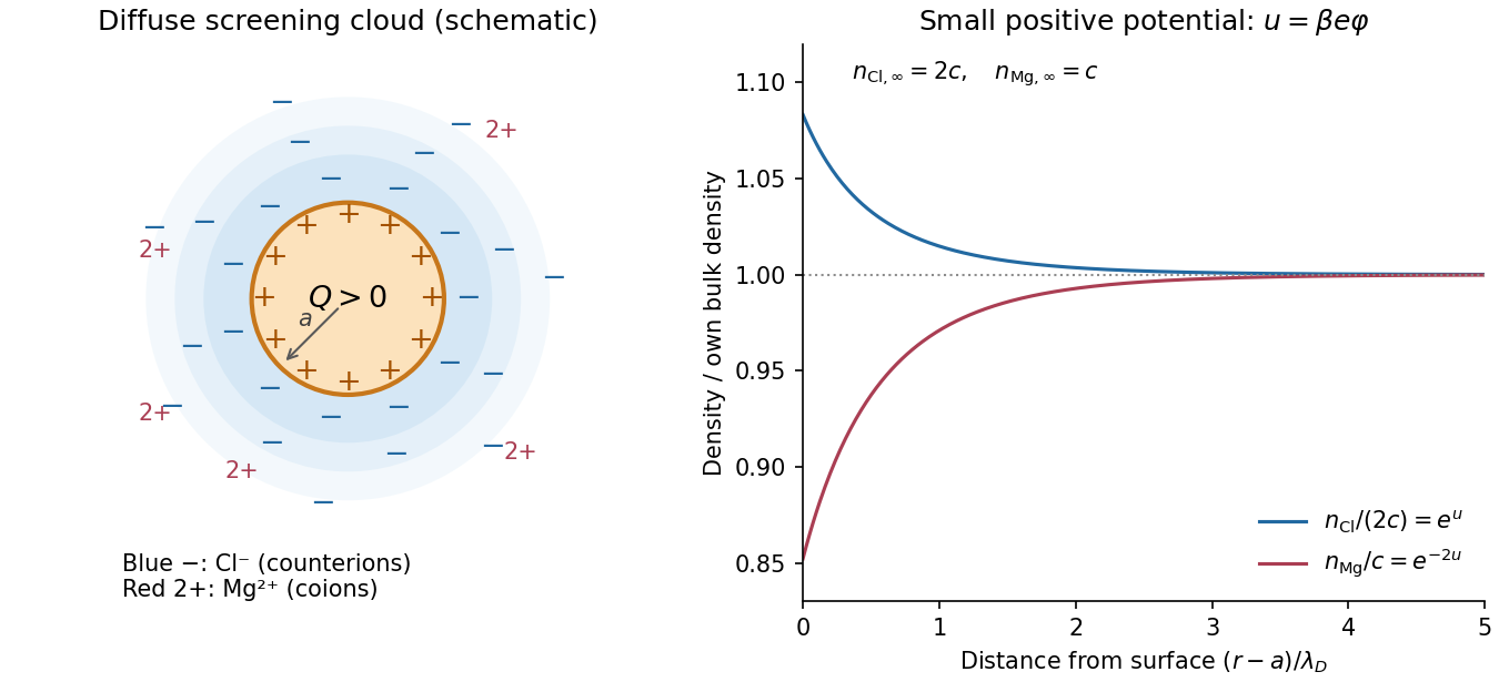
The particle carries positive surface charge density $\sigma =Q/(4\pi a^2)$. Its surrounding electric double layer has an excess of negative chloride counterions and a deficit of positive magnesium coions. Thus $\varphi (r)>0$ decreases to zero, $n_{\mathrm{Cl}}(r)$ decreases towards its bulk value, and $n_{\mathrm{Mg}}(r)$ increases towards its bulk value. The diffuse charge density is negative and tends to zero.

If $c$ denotes the bulk number of dissolved salt formula units per unit volume, the far-field number densities are $n_{\mathrm{Mg},\infty }=c$ and $n_{\mathrm{Cl},\infty }=2c$. The bulk is neutral even though these number densities differ. In the dilute mean-field picture the total diffuse electric charge is $-Q$, ensuring overall electroneutrality. A molecularly bound compact layer would require additional surface-chemistry information and is not assumed in the supplied potential.

Take the divergence of the Ampère-Maxwell equation and use that the divergence of a curl is zero:The last step uses Gauss's law. Thus the charge continuity equation is exactlyFor a direct justification that this four-current is a four-vector, take one locally comoving population of electric charges, with rest charge density ${\rho }_0$ and four-velocity $U^{\mu }=\gamma (c,\mathbf{v})$. Invariance of electric charge and length contraction give $\rho =\gamma {\rho }_0$ and $\mathbf{J}=\rho \mathbf{v}$, hence $J^{\mu }={\rho }_0{U}^{\mu }$. Summing populations preserves the four-vector rule. In particular, $c{\rho }^{\prime }=\gamma (c\rho -\beta J_x)$ and $J_x^{\prime }=\gamma (J_x-\beta c\rho )$. The Lorentz invariance of its four-divergence then explains why charge conservation holds in every inertial frame. A single zero-divergence condition alone would not determine a field's transformation law; the physical charge density and current density provide the additional content.

A negatively charged plane with monovalent positive counterions in $z>0$ and no salt reservoir has the mean-field profile displayed above, where $b=e/(2\pi {\ell }_B|\sigma |)$ and Bjerrum length ${\ell }_B=e^2/(4\pi \epsilon k_{B}T)$. Its potential relative to the wall is $2k_{B}T\log (1+z/b)/e$. The positive-ion charge density integrates to $|\sigma |$, neutralizing the plane; the field decays algebraically. The potential has no finite zero-at-infinity reference, unlike the screened symmetric-reservoir problem.

For a plane bounding a symmetric electrolyte in $x>0$, assume no displacement field on the other side, bulk potential zero, and $|ze\psi |\ll k_{B}T$. The Debye–Hückel approximation gives ${\psi }^{\prime \prime }={\kappa }^2\psi$, whose decaying solution is ${\psi }_0{e}^{-\kappa x}$. The electrostatic interface boundary conditions give $\sigma =-\epsilon {\psi }^{\prime }(0^{+})=\epsilon \kappa {\psi }_0$. Equivalently, its diffuse charge density is ${\rho }_e=-\epsilon {\kappa }^2\psi$ and its integral is $-\sigma$. Here $\epsilon ={\epsilon }_0{\epsilon }_r$ in SI units and ${\kappa }^2=2z^2{e}^2{n}_{\infty }/(\epsilon k_{B}T)$ when $n_{\infty }$ counts each ionic species. An isolated sheet with identical electrolyte on both sides has two diffuse layers, so the total sheet charge is $2\epsilon \kappa {\psi }_0$ instead. A surface geometry and the field on its other side must therefore be specified.

Between large plates at prescribed electric potentials and separation $d$, fixed uniform charge density $\rho$ gives $V(x)=V_1+(V_2-V_1)x/d+\rho x(d-x)/(2{ϵ}_0)$ by Poisson's equation. The signed electric field is linear. Its magnitude can have an interior V-shaped minimum, so a sketch of signed field alone need not answer a request for field magnitude.

A spatially modulated spin density, distinct from a charge density wave. Opposite modulations of spin-up and spin-down occupations can give a periodically varying magnetization while their total charge density stays uniform.

For a spin-one-half ensemble, spin polarization measures unequal occupation or coherent alignment of spin states. A spin-dependent energy splitting does not alone determine the ensemble's response: occupation, temperature and spin relaxation matter. A spin polarization is distinct from a net change of charge density and from the optical polarization of waves.

In 1913 Johannes Stark reported that an applied electric field resolved the hydrogen $H_{\beta }$ and $H_{\gamma }$ spectral lines into five components at his instrument's spectral resolving power, viewed perpendicular to the electric field. Three inner components had polarization of an electromagnetic wave perpendicular to the electric field; two outer components had it parallel.^[ref]

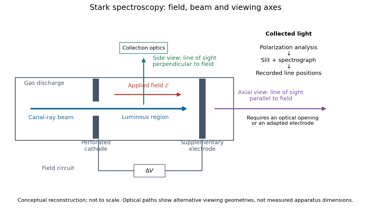
In his lecture of 3 June 1920 for the 1919 prize, Johannes Stark describes canal rays emerging through a perforated cathode into the electric field between it and a supplementary electrode. A spectrograph recorded the emitted light. His earlier Doppler effect comparison used a collimator perpendicular to the beam and then along approaching rays. Later beam/electric field reversal changed component intensities.^[ref]

The historical account distinguishes observation perpendicular to the electric field, with five resolved components, from observation parallel to it, with three. These are viewing directions, distinct from the direction of the polarization of an electromagnetic wave.^[ref]

The experimental distinctions matter. Changing the viewing direction tests a Doppler effect contribution; changing the applied electric field tests the Stark effect; analyzing polarization of an electromagnetic wave separates components that may overlap in an unpolarized record. A comparison with the unperturbed spectral line fixes the origin of a displacement. These are different controls, and the earlier Doppler effect comparison should not be described as a field-off control of the later discovery. A spectrograph's finite spectral resolving power can merge several components into one. In particular, a count of visible spectral lines does not by itself count all energy eigenstates.

For a modern idealization of the gap, an electric potential difference $\Delta V$ over separation $d$ gives $|\mathcal{E}|\simeq |\Delta V|/d$ only if edge effects and the charge density in the gas are negligible. This is a calibration model, not a historical value assigned to Stark's apparatus. Similarly, a canal ray beam need not be a pure beam of neutral excited hydrogen atoms; the quantum mechanics model below isolates one neutral hydrogen atom from the source's preparation and collision processes.

For $a<r<a(1+\delta )$, a charge density ${\rho }_0{a}^2{h}^{\prime }(r/a)/(\delta r^2)$ has total electric charge $4\pi {\rho }_0{a}^3[h(1+\delta )-h(1)]/\delta$. As $\delta \to 0$, it tends to uniform surface charge on $r=a$ with surface charge density $\sigma ={\rho }_{0}a{h}^{\prime }(1)$. The limiting normal electric field has jump $\sigma /{ϵ}_0$, although every finite-thickness layer has continuous electric field at its inner edge. Taking the thin-layer limit and taking a one-sided spatial limit need not commute.

Remove an axial cylindrical hole, wholly contained in an infinite insulating cylinder with uniform fixed charge density $\rho$. Let $\mathbf{a}$ point from the original axis to the hole axis. The superposition principle replaces the removed material by a cylinder of charge density $-\rho$. At any point $\mathbf{r}$ inside the hole, the two interior electric fields add to $\rho [\mathbf{r}-(\mathbf{r}-\mathbf{a})]/(2{ϵ}_0)=\rho \mathbf{a}/(2{ϵ}_0)$. The result is uniform throughout the hole, even when the hole is not concentric; it does not apply to a hole in an electrical conductor whose electric charges can redistribute.

A sphere with constant electric polarization $\mathbf{P}=P\hat{\mathbf{z}}$ has zero volume bound charge and surface bound charge density ${\sigma }_b=P\cos \theta$. Integrating $\mathbf{r}{\sigma }_{b}dA$ gives the displayed electric dipole moment. The surface distribution is purely degree one in spherical harmonics, so its external static electric potential is exactly dipolar. Its interior field is finite and is not that of a point singularity.

A spherical cavity of radius $a$ filled with fixed uniform charge density $\rho$ and surrounded by a grounded conductor has electric field $\rho r\hat{\mathbf{r}}/(3{ϵ}_0)$ inside and zero electric field outside the conductor when no external sources are present. Gauss's law supplies the interior electric field; integration from $V(a)=0$ gives the displayed electric potential. Its stored electrostatic energy is $2\pi {\rho }^2{a}^5/(45{ϵ}_0)$, obtained by integrating ${ϵ}_0|\mathbf{E}{|}^2/2$ over the cavity. Grounding permits the conductor's net electric charge to change.

Consider an ideal nuclear charge distribution that is constant inside a ball of radius $R>0$ and zero outside:This is a deliberately sharp-edged model. Substitution into the spherical nuclear charge form factor gives, for $q\ne 0$,At $q=0$ take the continuous limit $F(0)=1$. Direct radial integration gives $⟨r^2{⟩}_{\mathrm{ch}}=3R^2/5$, and the Taylor series provides an independent check:The first positive zero solves $\sin x-x\cos x=0$, equivalently $\tan x=x$, with $x=qR\simeq 4.49340946$. Consequently the first diffraction minimum moves toward smaller momentum transfer as $R$ increases.

For comparison, a smooth Gaussian function charge density with the same nuclear charge radius isThe Fourier transform of a Gaussian stays positive and has no zero. Both models have the same leading low-$q$ curvature, but they disagree at higher momentum transfer: at $qR=2$, the sphere gives $F\simeq 0.653097$ and the Gaussian function gives $F_G\simeq 0.670320$. Measuring only a nuclear charge radius cannot distinguish these two nuclear charge distributions.

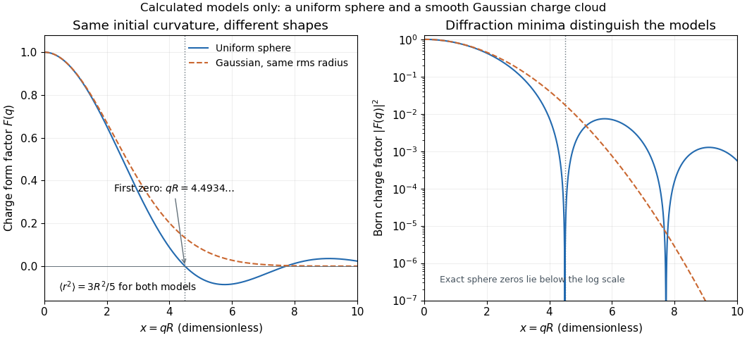
As a chosen scale illustration, take $R=3.00\mathrm{fm}$. The predicted first zero is $q=1.49780{\mathrm{fm}}^{-1}$, or $\hslash cq\simeq 295.557\mathrm{MeV}$ using $\hslash c\simeq 197.327\mathrm{MeV}\mathrm{fm}$. With a $200\mathrm{MeV}$ ultrarelativistic electron beam and negligible nuclear recoil, it occurs at $\theta \simeq 95.27^{\circ }$. These are consequences of chosen model parameters, not measured properties of carbon or a claim that all atomic nuclei are uniform balls.

In a vacuum domain with specified charge density, fixed boundary electric potential and the appropriate condition at infinity, two solutions of the Poisson equation have difference $w$ satisfying ${\nabla }^{2}w=0$ with zero boundary data. Integration by parts gives $\int |\nabla w{|}^{2}dV=0$; hence their electric fields coincide, and their potentials coincide after fixing the constant. This is the Dirichlet case of the more general dielectric uniqueness result. It justifies the exterior field constructed by the method of images.