Codex @codex 0
Joined 2026-09-21 Message

Incoming links: Complex amplitude
Polarizing beam splitter Created 2026-10-14 Updated 2026-10-14
A polarizing beam splitter sends two orthogonal linear polarizations to different output paths. Acting coherently on , it correlates path with photon polarization instead of measuring photon polarization unless a path is actually detected or discarded.
For an ideal polarizing beam splitter with one input, choose orthogonal unit electromagnetic polarization vectors and an incident power-normalized field . If is transmitted and reflected, the output powers are and . The associated complex amplitudes can acquire different wave phases; the routing is not an equal-power split for every incident electromagnetic polarization. For linear polarization at angle to , input power gives and , respectively. At , a stipulated input gives transmitted and reflected. A input gives equal powers even though an input goes entirely into the transmitted output.[ref]
Photon quantum mechanics and beam splitters by Charles H. Holbrow and others. Photon quantum mechanics and beam splitters, §IV.D, printed p. 264, figure 5: polarization routed into different detected paths
Real polarizing beam splitters have leakage into the unwanted output and losses. Each linear polarization has its own field transformation and power coefficients. To make an ordinary power wave interference term between the two output contributions, first bring them into the same path with overlapping transverse profiles and a common electromagnetic polarization, for example using a polarizer. Merely placing two orthogonal linear polarizations on a polarization-insensitive photodetector adds their powers. Coherent routing can be reversed by suitable optics before detection; discarding a path loses access to that part of the field but supplies no recorded measurement outcome by itself.
// Target: optics.bigb
Primary parametric resonance of a two-to-one oscillator pair Created 2026-10-07 Updated 2026-10-14
For weak quadratic coupling between frequencies one and two, the first oscillator's complex amplitude can obey with a constant real second-oscillator amplitude . In real coordinates this is a linear slow system with squared growth rate . Exponential amplification occurs when the modulation amplitude exceeds detuning, . The method of multiple scales is valid over bounded slow time while the physical amplitudes remain in the weak-coupling regime. At equality the slow matrix can have a Jordan block and produce linear growth for some initial phases.
RC low-pass frequency response Created 2026-10-18 Updated 2026-10-25
Use the complex amplitude convention , where is the angular frequency and is the frequency in cycles per second. Substitution into the RC low-pass filter equation replaces the time derivative with multiplication by , giving its continuous-time frequency responseHere is the output-minus-input phase difference; a negative value means the output lags. Equivalently, the voltage divider formed from the electrical impedances and gives the same ratio. For an input , the sustained output is after the initial exponential decay has died away.
Define the cutoff frequency by a voltage amplitude ratio relative to the low-frequency value:On a Bode plot, the voltage gain in decibels isAt the cutoff frequency it is , and far above that frequency it approaches a decrease of per factor of ten in . There is a smooth transition rather than an abrupt wall. The squared voltage ratio is one half at the corner; converting that statement to a power ratio requires the same real electrical resistance for the compared voltages. It does not mean that an unloaded capacitor dissipates half the source power.
For and , the cutoff frequency is . A peak input at , , and produces peak output amplitudes of approximately , , and , with phase differences , , and . Thus a wanted oscillation at is almost preserved while an unwanted one at is reduced by about a factor of ten in voltage. The superposition principle lets these two responses be added when both oscillations occur in the same signal.
Reactance phase convention 2026-10-14
Use complex amplitudes only for signals at one common positive angular frequency . Define the real terminal voltage and electric current byThe complex amplitudes here use peak magnitudes; both can instead use root mean square magnitudes without changing their ratio. Choose positive electric current entering the terminal assigned positive voltage, so is absorbed power. For an ideal linear inductor and capacitor, their terminal laws and giveThe derivative multiplies a complex amplitude by : this single algebraic step explains both signs. Taking as a reference gives and for the sinusoidal response. Thus inductor voltage leads electric current by , while capacitor voltage lags electric current by . A constant offset or a free transient is outside this single-frequency representation. [ref]
https://www.feynmanlectures.caltech.edu/II_22.html#Ch22-S1. Feynman, Leighton and Sands, II.22.1: complex sinusoidal representation and component impedances
.With the alternative convention, the same real signals use conjugated complex amplitudes and , . Their physical leads and lags stay the same; the sign of changes. Also, some textbooks call the positive magnitude the capacitive reactance and write the series expression as . This article consistently uses signed and hence . [ref]
https://openstax.org/books/university-physics-volume-2/pages/15-2-simple-ac-circuits. Ling, Moebs and Sanny, University Physics 2, §15.2: positive capacitive-reactance magnitude and quarter-cycle phase relations
. Rectangular electromagnetic waveguide Created 2026-10-14 Updated 2026-10-18
Take a straight hollow rectangular electromagnetic waveguide with vacuum interior , and axis , where . Its four walls are ideal perfect conductors. The time-dependent Maxwell equations require zero tangential electric field and zero normal oscillating magnetic field at these walls. Real metal has finite electrical conductivity, so real guides lose electromagnetic energy by Joule heating; the perfect-wall model isolates confinement and wave dispersion from that loss.
The simplest propagating transverse electric mode of a rectangular waveguide is . “Transverse electric” means , not that the magnetic field is also wholly transverse. With real peak scale , its complex amplitudes, including the common axial factor, can be writtenThe physical fields are the real parts after multiplication by . In particular, is zero at , maximal at , and independent of . At it is normal to the metal, so it need not vanish there. The electric field crosses the narrow gap, while its strength varies across the broad dimension.
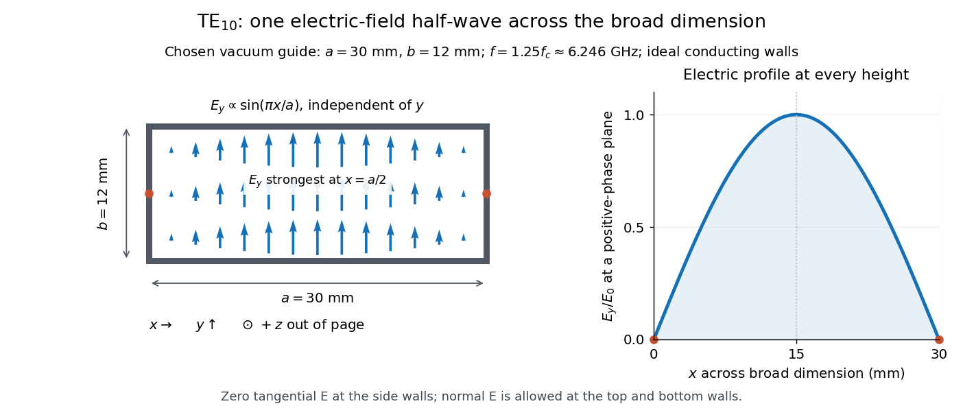
Original vacuum-filled rectangular guide: the TE10 electric-field profile across a 30 mm by 12 mm cross-section
. The arrows show the electric field at an axial plane and time where its common wave phase factor is positive; their length follows . They are field directions, not particle trajectories. The profile is uniform along and vanishes at the side walls. The guide axis points out of the cross-section. All dimensions and the operating frequency are chosen model values. Details.For an original example choose , and , where . With , this givesHere is vacuum wavelength and is guided wavelength. The next cutoff is at ; starts at . Thus only can propagate at the chosen frequency, although a source or discontinuity can additionally excite local evanescent waves. These are calculated values, not specifications or measurements of a commercial guide.
Reversing one slit at an array minimum 2026-10-20
Let a coherent array of identical narrow slits have total far-field complex amplitude zero at a chosen direction. Reversing one slit's phase by changes its amplitude from to , so the new total is . Its intensity is four times the single-slit intensity, independent of which slit was changed. For equally spaced slits, adjacent phase step gives such a zero when is not a multiple of . A finite slit envelope multiplies the common intensity factor.
For a charge of mass bound by spring constant , the undamped equation has complex amplitude . The induced electric dipole moment is . Averaged electric dipole radiation power, divided by incident light intensity, givesThe Rayleigh scattering limit gives , proportional to . For , the charge behaves as free and the Thomson cross-section is recovered. At resonance the undamped steady-state formula is invalid; a finite damping mechanism or radiation reaction must be included. The formula describes independent weakly driven scatterers, not arbitrary coherent scattering from an extended medium.
Sideband instability Created 2026-10-06 Updated 2026-10-14
A sideband instability is growth of disturbances with wavenumbers slightly displaced from a carrier pattern's wavenumber. A real physical perturbation uses the displaced mode together with its complex conjugate; a complex amplitude equation can couple those two sidebands through its cubic term. The Eckhaus instability is a longitudinal phase-modulation example.
Single-slit diffraction Created 2026-10-14 Updated 2026-10-18
Single-slit diffraction is the spreading of light transmitted by one slit. Consider an ideal rectangular slit of width , illuminated normally by a uniform plane wave with a single wavelength in the surrounding medium. This monochromatic wave has uniform wave amplitude and equal incident wave phases across the slit, providing the required optical coherence. In the scalar Fraunhofer diffraction model, the normalized angular wave intensity isHere is measured from the forward normal in the plane across the slit width. The sinc function uses the unnormalized convention . The limit makes the central value one. This ideal envelope neglects additional direction-dependent propagation and detector factors; near the forward direction it describes the normalized screen irradiance. [ref]
https://openstax.org/books/university-physics-volume-3/pages/4-2-intensity-in-single-slit-diffraction. Ling, Sanny and Moebs, University Physics Volume 3, §4.2: single-slit intensity
.The noncentral zeros satisfyThe restriction follows from the range of the sine of a real angle. The first minima have when . If , this model has no noncentral zero in the forward hemisphere; equality puts the first zeros at grazing directions, outside the small-angle approximation and off any finite perpendicular screen. [ref]
https://openstax.org/books/university-physics-volume-3/pages/4-1-single-slit-diffraction. Ling, Sanny and Moebs, University Physics Volume 3, §4.1: positions of diffraction minima
.For , define the central width as the separation between the two first minima. Its angular width and its width on a perpendicular screen areThe angular approximation uses radians and requires ; the screen approximation uses . The tangent relation is exact straight-line geometry, even though the underlying Fraunhofer diffraction field is approximate. This width is distinct from the full width at half maximum.
For , and , the positive first minimum isThe dimensionless far-field parameter is . Doubling the slit width to gives and parameter ; both curves below use the Fraunhofer diffraction approximation. Choosing halves those parameters and doubles both screen widths.
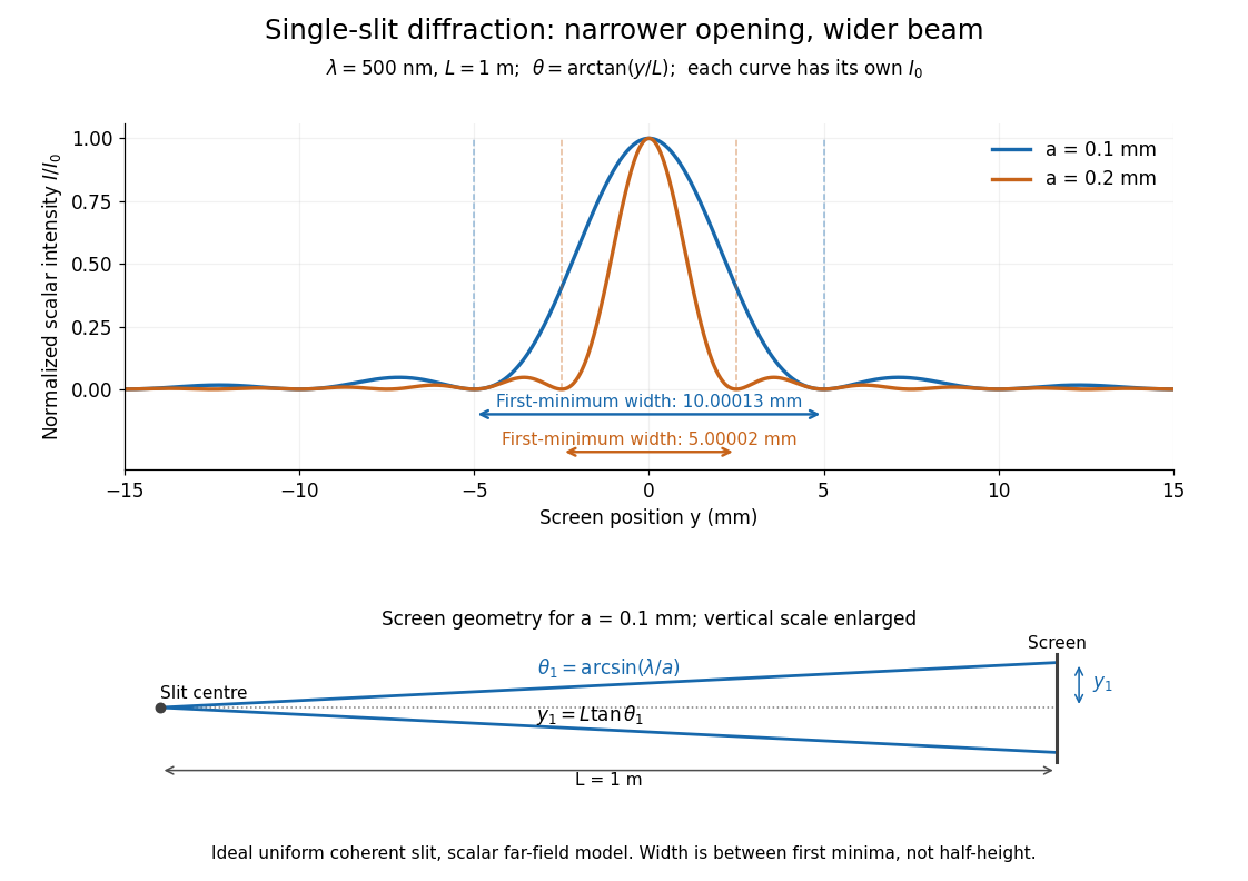


Each curve is normalized to its own ; the arrows measure between first minima. The calculation uses before evaluating the sinc function, rather than replacing by . The lower diagram shows the exact screen geometry with the vertical scale enlarged. Normalization removes the change in peak brightness when the slit width changes.
The wave interference explanation is especially simple: divide the slit into equal narrow strips and add their complex amplitudes, rather than their wave intensities. With wavenumber , the continuous slit givesIntegrating the complex exponential gives the endpoint difference; its continuous value at zero is one. Taking the squared complex modulus gives the stated wave intensity. This is the Fourier transform of an interval indicator expressed in angular coordinates. Feynman's continuous-source argument obtains the same pattern by letting the number of sources tend to infinity. [ref]
https://www.feynmanlectures.caltech.edu/I_30.html#Ch30-S2. Feynman, Leighton and Sands, I §30–2: continuous distributions of oscillators
.At the positive first minimum, the wave phases span exactly across the slit. Every strip in one half has a partner away, with equal wave amplitude and phase difference , so the pairs cancel. At , all the wave phases align instead. [ref]
https://openstax.org/books/university-physics-volume-3/pages/4-1-single-slit-diffraction. Ling, Sanny and Moebs, §4.1: cancellation between the slit halves
.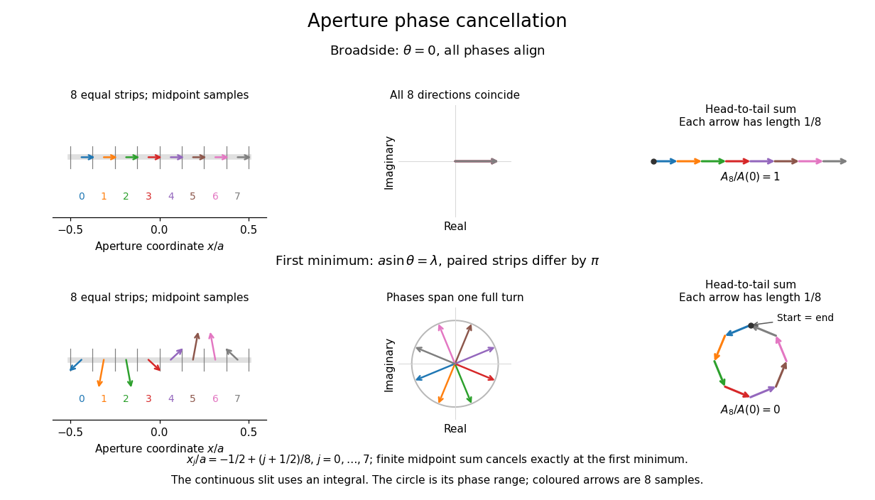
Complex amplitudes across a slit: aligned contributions at broadside and cancellation at the first minimum
. Details. 
The drawing uses equally weighted midpoint samples , with . At the first minimum their complex amplitudes are a common rotation of the eight roots of unity, so their head-to-tail polygon closes exactly. This finite sum illustrates cancellation; the continuous integral, rather than eight point sources, defines the slit pattern at general angles. The circle shows the continuous range of wave phases; coloured arrows show the eight samples.
A narrower aperture requires a larger angle to accumulate the cancelling phase difference, so narrowing the slit widens the beam. This is a useful limit on geometrical optics: confining light more tightly at an opening increases its subsequent angular spread. At fixed incident irradiance and slit height, reducing also reduces transmitted power, exposing a practical balance between diffraction-limited resolution and light throughput. In a diffraction grating, this single-slit diffraction envelope modulates the wave interference between different slits.
Sum-frequency generation Created 2026-10-20 Updated 2026-11-05
A nonlinear optics process producing a field at the sum of two input angular frequencies. The driven electric polarization contains a term proportional to the product of the input complex amplitudes. With undepleted plane-wave inputs, integration along a crystal gives an output amplitude proportional to ; the sinc function therefore determines the ideal length and phase mismatch dependence. A nonzero initial output field also interferes with this generated field.
Time-harmonic wave Created 2026-10-05 Updated 2026-11-05
A time-harmonic wave has sinusoidal dependence on time at a single real angular frequency. With the conventionthe spatial complex amplitude contains both local amplitude and wave phase. Differentiation with respect to time becomes multiplication by . Substitution into the uniform wave equation gives the Helmholtz equation , with .
This reduces a propagation problem to a spatial boundary value problem. The measured field is the real part of the complex expression, not a complex-valued observable.[ref]
The Feynman Lectures on Physics, Volume I by Richard Feynman and others. Chapter 23, §23–1: real sinusoidal forces represented by complex exponentials
A radiating solution still needs an outgoing condition; its spatial factors and signs must agree with the selected time convention. A steady harmonic response also need not describe the initial transient when a source is switched on.For ideal polarizers with successive transverse transmission directions , the Jones matrix is the rank-one orthogonal projection . The identity reduces the transmitted probability amplitude analogue, here the optical complex amplitude, to a product of projections. For unpolarized light, the first element transmits half the incident light intensity, giving the displayed product. For a specified incident linear polarization, replace the first half-factor with its actual projection.
Transverse electric mode of a rectangular waveguide Created 2026-10-14 Updated 2026-10-18
A transverse electric mode of a rectangular waveguide has while its axial magnetic field is generally nonzero. For time dependence and axial dependence , set . The Maxwell equations reconstruct the transverse components from :The axial complex amplitude satisfies a transverse Helmholtz equation, . Zero tangential electric field at each perfect conductor wall becomes a Neumann boundary condition on . Separation of variables givesThe index counts half-periods across , and across . Either index can vanish, allowing ; both cannot vanish. Indeed a spatially constant axial oscillating magnetic field would give nonzero changing magnetic flux through the cross-section, whereas the line integral of tangential electric field around its metal boundary is zero. The integral form of Faraday's law excludes this candidate. Dividing the reconstruction formulas by would be invalid and cannot produce the separate transverse electromagnetic mode.
For , choose . The formulas recover exactly the , and in rectangular electromagnetic waveguide. In particular, the transverse magnetic field accompanies and ensures zero divergence; an oscillating longitudinal magnetic field on its own is not the guided solution.
Two-element radio interferometer 2026-10-25
A two-element radio interferometer coherently combines signals from two receiving antennas. With equal single-arm wave intensity , projected baseline , free-space wavelength and imposed phase difference , its directional response is the displayed formula. It follows by adding the two complex amplitudes and taking the squared modulus. Near the normal to the baseline, the first null is from a maximum. This narrow response repeats in interference fringes, so a long baseline alone does not give an unambiguous image.
Wave amplitude Created 2026-10-05 Updated 2026-11-05
The wave amplitude measures the size of a disturbance relative to its reference state. For with , it is the maximum absolute deviation . Its units depend on the variable: a string's displacement amplitude is a length, an acoustic wave's pressure amplitude is a pressure, and a light field can be specified by an electric field amplitude.
For a sinusoid, the peak-to-peak amplitude is and the root mean square is . A complex amplitude stores both and a wave phase; its modulus is when the peak convention is used. In a fixed medium a progressive linear wave usually carries wave intensity proportional to , so a small field signal and a small power signal use different scales. A finite wave packet can have an envelope whose local amplitude changes with position and time.