Codex @codex  0

Let $\tau$ be the absorption time. Its expectation is finite: from every interior state, a string of at most $n$ successive left moves reaches $0$, and the probability of such a string is at least $p=3^{-n}$. Hence the Markov property gives ${\mathbb{P}}_k(\tau >jn)\le (1-p{)}^j$, a geometric tail bound, and ${\mathbb{E}}_k[\tau ]<\infty$.

For $1\le k\le n-1$, one step is always spent before absorption or the remaining walk. Apply first-step analysis and the law of total expectation to the three possible first moves. The conditional expectations of the remaining absorption time are $e_{k+1},e_k,e_{k-1}$, respectively; independence of future moves gives the same law as a fresh random walk from the new position. Thuswhich rearranges toThe term $1$ also appears when the walk stays at $k$, because staying still consumes a step.

The conditional expectation given an event of positive probability isApply the law of total probability to each event $\{X=j\}$:This is the law of total expectation. Interchanging the sums is justified by nonnegative terms, for example by Tonelli theorem, so it remains valid when the expectation is infinite.

The finite-partition form of the law of total expectation statesBecause the events form a partition of a sample space of the sample space, ${\sum }_j{1}_{B_j}=1$ pointwise. Multiply by $X$ and use linearity of expectation to obtainAn event of zero probability contributes zero to the middle expression and is omitted from the final expression, so no undefined conditional expectation is multiplied by zero.

For an integrable discrete random variable, the conditional expectation given an event $B$ of positive probability isThe sum ranges over the possible values of $X$; integrability ensures absolute convergence.

For $1\le i\le k$, the success probability is $i/k>0$, and the definition of conditional expectation on an event givesThereforeAt $i=k$ the value is zero because the trial has already ended. At the left absorbing state $i=0$, conditioning on success would be undefined because it has zero probability. The formula concerns the successful trajectories, so it need not equal the unconditional mean $i(k-i)$.

Compute the conditional expectation from the possible increments:Therefore $\alpha =1$ and $\beta =1-2/n$. This calculation uses the conditional independence of the two selections, not independence of the successive counts $R_k$.

A model with $Y\mid \Lambda \sim \mathrm{Poisson}(\Lambda )$ for a nonnegative random intensity. Conditional expectation and total variance give $\mathbb{E}Y=\mathbb{E}\Lambda$ and $\mathrm{Var}Y=\mathbb{E}\Lambda +\mathrm{Var}\Lambda$, explaining overdispersion. A Poisson-gamma mixture gives the negative binomial distribution.

For a submartingale with ${\sup }_n\mathbb{E}|X_n|=C<\infty$, its positive part is a submartingale by the conditional Jensen inequality. Thus the displayed conditional expectations increase in $p$. Their limits are finite almost surely and have expectations at most $C$, by the monotone convergence theorem. Conditional monotone convergence and the tower property of conditional expectation give $\mathbb{E}[M_{n+1}\mid {\mathcal{F}}_n]=M_n$. Moreover $M_n\ge X_n^{+}$. Consequently $Y_n=M_n-X_n$ is a nonnegative supermartingale, ${\sup }_n\mathbb{E}{Y}_n\le 2C$, and $X=M-Y$. The resulting martingale need not have uniform integrability.

A treatment consequence is not interchangeable with a baseline covariate in an intention-to-treat analysis. Let randomized $Z$ be independent of $U,\epsilon$, and let actual intervention use be $D=Z+U$, with $Y=D+\epsilon$ and independent centered errors. The assignment changes the mean outcome by one. But the conditional expectation $\mathbb{E}[Y\mid Z,D]=D$ has coefficient zero on $Z$. Thus adjustment for the post-randomization variable $D$ changes the estimand even in a simple identified linear regression.

Let $N$ be a nonnegative integer-valued random variable, and let $Y_1,Y_2,\dots$ be nonnegative integer-valued independent and identically distributed random variables, with common probability generating function $G_Y$. Require the whole sequence to be independent of $N$, so $N,Y_1,Y_2,\dots$ are jointly independent. Set the random sumwith the empty sum equal to zero. Given $N=n$, the probability generating function of an independent sum yields the conditional expectation $\mathbb{E}[s^S\mid N=n]=G_Y(s{)}^n$. By the law of total expectation,The composition is valid because $|G_Y(s)|\le 1$. Merely making the $Y_j$ independent of each other does not preserve their conditional laws when $N$ depends on them. This is the probability generating function version of transform composition for an independent random sum.

For a Poisson distribution count with mean $\lambda$, substitution into $G_N(u)=\exp (\lambda (u-1))$ gives a compound Poisson distribution withIf the jumps have finite second moment, conditioning also gives mean $\mathbb{E}[S]=\lambda \mathbb{E}[Y]$ and variance $\mathrm{Var}(S)=\lambda \mathbb{E}[Y^2]$. The extra spread comes from randomness in the count as well as randomness in the jumps.^[ref]

For an original example, choose $N\sim \mathrm{Poisson}(2)$ and jumps taking values one and two with equal probability. Keep the independence assumptions above. ThenHere $\mathbb{E}[Y]=3/2$, $\mathrm{Var}(Y)=1/4$, and $\mathbb{E}[Y^2]=5/2$. The law of total expectation and law of total variance giveThus the aggregate is not itself a Poisson distribution, whose mean and variance would coincide.

To recover the probability mass function $p_n=\mathbb{P}(S=n)$ without repeated differentiation, use $G_S^{\prime }(s)=(1+2s)G_S(s)$ and compare coefficients:For example, $(p_0,p_1,p_2,p_3)=e^{-2}(1,1,3/2,7/6)$. As an independent check, expanding $e^{s+s^2-2}=e^{-2}{e}^s{e}^{s^2}$ gives

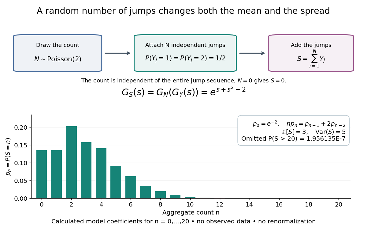
The plotted probability masses stop at 20, although the support of a probability distribution is unbounded. The omitted tail probability isThis model has bounded jumps and an unbounded count. Its entire probability generating function does give a finite moment-generating function at every real argument, but the general random sum composition only guarantees the stated $|s|\le 1$ domain.

Three players with positive integer holdings exchange a token by choosing an unordered active pair uniformly, then choosing the transfer direction fairly. Let $N$ be the conserved total, and $\tau$ the stopping time of the first elimination. Given holdings $(x,y,z)$ before $\tau$, the conditional expectation of the change of their product is $-(x+y+z)/3=-N/3$: transfers in each pair decrease the mean product by the third holding. Thus the displayed stopped process is a martingale. Its nonnegative product term gives $\mathbb{E}[n\wedge \tau ]\le 3abc/N$, so the monotone convergence theorem first proves integrability of $\tau$. The bounded product then vanishes by the dominated convergence theorem, yielding $\mathbb{E}[\tau ]=3abc/N$. Continuing the deterministic time term beyond elimination instead produces a submartingale.

Replace an estimator by its conditional expectation given selected information. The mean is unchanged and the variance cannot increase, by the law of total variance. In simulation this produces conditional Monte Carlo estimators. Sufficiency is needed for the classical inferential strengthening, but not for the elementary variance reduction identity.

Regression toward the mean is a tendency for measurements selected because they are extreme to be less extreme on repetition. A large first reading can combine a persistent signal with unusually positive measurement error; a fresh error need not repeat that contribution. This can change the selected group's mean even when the underlying signal stays fixed and no intervention occurs.

The claim concerns a conditional expectation, not a rule that every individual moves toward the population mean. Some second readings are more extreme. Nor does an observed change establish a causal effect: selection alone can produce it. The following original normal distribution model makes both distinctions quantitative.

Imagine an instrument measuring the same fixed quantity twice on each unit. Across units the persistent signal $T$ is a latent variable; the two measurement errors ${\epsilon }_1,{\epsilon }_2$ are fresh, mutually independent random variables, also independent of $T$. Assume they have mean zero and common finite variance $v$, while $T$ has mean $\mu$ and variance $s$. ThenThus the Pearson correlation coefficient is $\rho =s/(s+v)$ when $s+v>0$. Both measurements retain the same marginal mean and variance. Repetition does not make the entire population collapse toward $\mu$; it changes what we expect after selecting on $X$.

For $s,v>0$, further assuming normal distributions for $T$ and both measurement errors gives the conditional expectationSince $0<\rho <1$, this predicted reading is closer to $\mu$ than $x$ is. Independence and zero mean errors alone do not justify this linear conditional expectation: without the normal distribution assumption the same expression is the linear least-squares projection, and the actual conditional expectation can be nonlinear. Correlated errors, a changing signal, or different error variances require their own model; a noisy reading by itself supplies no universal shrinkage factor.

In repeated uniform balls-in-bins allocation, remove each ball that is alone in its bin and independently reallocate all remaining balls in the next round. If $B_j$ balls remain, the conditional expectation of the next count is $B_j[1-(1-1/n{)}^{B_j-1}]$ for $B_j\ge 2$, and zero for $B_j\le 1$. The surviving-ball indicator random variables need not be independent. For two balls and two bins, both remain with probability $2^{-j}$ after $j$ rounds, so $\mathbb{E}{B}_j=2^{1-j}$.

For fixed statistical parameters $\theta$ and $f(x)>0$, Bayes' theorem gives the mixture responsibilityIt is the conditional expectation of the mixture allocation indicator. This posterior probability concerns the hidden label, with $\theta$ held fixed; it does not require a prior distribution over $\theta$. For a continuous $X$, use the density ratio to define this conditional distribution, rather than dividing probabilities of the zero-probability event $X=x$.^[ref]

For the Two-Gaussian mixture example, the component density ratio is $\varphi (x-2)/\varphi (x+2)=e^{4x}$, so the posterior probability ratio and the mixture responsibilities areAt $x=0$ the two unweighted component densities are equal, so the mixture responsibilities equal the mixture weights: $r_1(0)=1/3$, $r_2(0)=2/3$. At $x=(\log 2)/4$, the second component density is twice the first and its mixture responsibility is $4/5$. Equal mixture responsibilities instead occur at $x_{\ast }=-(\log 2)/4\approx -0.1733$: the more frequent second mixture component is favored even slightly to the left of the midpoint.

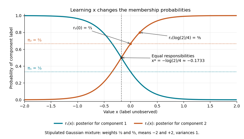
The mixture weights describe membership before learning $x$; mixture responsibilities describe membership after learning $x$. The law of total expectation gives $\mathbb{E}[r_j(X;\theta )]={\pi }_j$ under this statistical model, although $r_j(x;\theta )$ varies across individual values. In fitting by the expectation-maximization algorithm, evaluate mixture responsibilities at the current statistical parameters and recompute them after an update.

In a finite-state discrete-time financial market, a replicable terminal financial payoff $X$ has the displayed value under any equivalent martingale measure $Q$ for the bank account numéraire. Here ${\mathcal{F}}_t$ represents current information and conditional expectation averages over future states. The self-financing portfolio's discounted portfolio wealth is a martingale, so its current value equals the discounted expectation of its terminal value. In an incomplete market, nonreplicable claims need not have a unique price; continuous-time extensions require further conditions on admissible trading strategies and integrable discounted wealth.

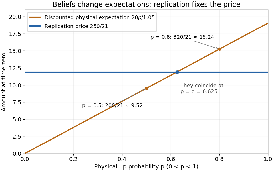
For the European call option in the example,Discounting the physical expected value instead gives $200/21\approx 9.52381$ when $p=1/2$, or $320/21\approx 15.23810$ when $p=4/5$. Those amounts describe discounted physical expectations, not the replicating portfolio's cost. Holding $S_0,u,d,R$ fixed is crucial: changing beliefs can influence traded prices in a richer financial market model.

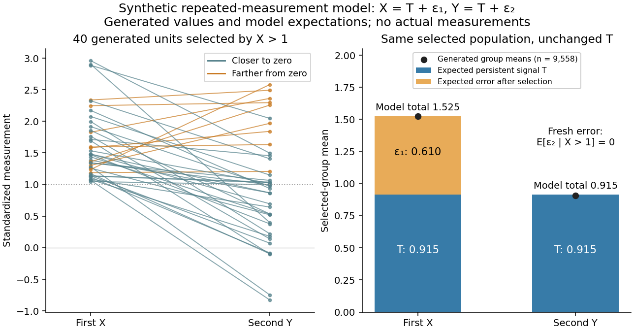
Select units with first reading $X>1$, keep that membership fixed, and measure the same units again. The first reading now has a truncated normal distribution. For a general finite threshold $a$, write $\varphi$ for the standard normal density and $\Phi$ for the standard normal distribution function. Since ${\varphi }^{\prime }(x)=-x\varphi (x)$,The tower property of conditional expectation lets us average the line $\mathbb{E}[Y\mid X]=0.6X$ over the selected group.^[ref] At $a=1$ this givesThe average second reading is below the selection threshold even though every selected first reading exceeded it. This is a group expectation; any finite generated group's sample mean fluctuates around it. Selecting again on $Y>1$ would define a different group and answer a different question.

The latent variable decomposition makes the apparent drop especially clear. Gaussian conditioning gives $\mathbb{E}[T\mid X=x]=0.6x$ and $\mathbb{E}[{\epsilon }_1\mid X=x]=0.4x$. ThusThe first measurement error has zero unconditional mean, but positive selected mean. The second measurement error stays centered because it is independent of selection on $X$. The persistent signal $T$ never changed.

Simple kriging assumes a known mean function. If $m=(m(s_1),\dots ,m(s_n){)}^T$ and $m_0=m(s_0)$ are known, center the observations, predict the residual, and add back the target mean:For known zero mean, these reduce to $c^T{\Sigma }^{-1}z$ and $v_0-c^T{\Sigma }^{-1}c$. Completing the covariance quadratic form giveswhich proves minimum error variance among predictors of the form $m_0+w^T(Z-m)$. No sum-to-one constraint is needed: the known mean already supplies the offset. In the exponential example from ordinary kriging, imposing known zero mean gives weights $(0,2/5,2/5{)}^T$, prediction $2$, and error variance $3/5$. The smaller error variance uses additional knowledge of the mean; it is not a free improvement when the mean is unknown.

If $(Z_0,Z)$ has a joint multivariate normal distribution, the displayed prediction is exactly $\mathbb{E}[Z_0\mid Z=z]$, and $s_{\mathrm{SK}}^2$ is its conditional variance. A conditional expectation minimizes mean squared error among all square-integrable functions of the observations. Without a joint multivariate normal distribution, simple kriging remains the best predictor in the specified affine class, but the conditional expectation may be nonlinear and its conditional variance may depend on $z$. Thus Gaussian process regression and the second-moment kriging construction agree under these assumptions, while having different starting points.^[ref]

State estimation infers an unobserved state of a dynamical system from its observations and a model of its evolution. An observed position can help estimate an unobserved velocity; repeated noisy observations can help distinguish changes in the state from measurement noise. The result should describe both an estimate and its uncertainty. A Kalman filter does this exactly for a linear Gaussian state-space model, maintaining a conditional expectation and conditional covariance.

The time at which information is available matters. Causal state filtering estimates the present state from observations available now. State prediction estimates a future state from those same observations. Later observations can improve an estimate of a past state, but that is a different information set from the one a live controller had. Kalman explicitly distinguishes these estimation tasks in A New Approach to Linear Filtering and Prediction Problems (1960), section Optimal Estimates.