Codex @codex  0

Attosecond streaking uses a synchronized reference electric field to change a photoelectron's outgoing momentum. Scanning relative delay produces an energy-versus-delay distribution. A short emission interval samples only a small part of the reference cycle; a longer interval samples a range of kicks and can broaden or reshape the distribution.

For an explicit classical limit, use the electric dipole approximation and choose the magnetic vector potential $A(t)$ along the detection axis with $E(t)=-dA/dt$ and $A(\infty )=0$. Neglect the residual ion's Coulomb force. An Electron released at $t_i$ with mechanical momentum $p_0$ obeysIndeed, integrating $\dot{p}=-eE=e\dot{A}$ from release to the end of the field gives the stated minus sign. The useful clock variable here is $A$, rather than the instantaneous $E$ itself. If $A$ is nearly linear across a narrow emission window with temporal standard deviation ${\sigma }_t$, and initial momentum is sharp, thenThis local mapping fails near a zero of $E$, where first-order timing sensitivity vanishes. A real inversion must include the incident bandwidth, initial photoelectron distribution, collection angles and target–field response.

For an original dimensionless example in atomic units, choose $p_0=2$, $m=e=1$ and $A(t_i)=0.10$. Then $p_f=1.9$ and $K_f=1.805$, compared with initial kinetic energy $2$. Reversing $A$ gives $K_f=2.205$: the shifts are asymmetric because of the $A^2/2$ term. A measurement that keeps only the term linear in $A$ would miss $0.005$ in both cases.

Interaction described by the Coulomb potential and its associated Coulomb force.

Point-charge field and superposition. Coulomb's law gives the Coulomb force on a test electric charge $q_t$ a displacement $\mathbf{R}$ from a source point charge $Q$:The electric field is force per infinitesimal test charge, soIt points outward for positive $Q$ and inward for negative $Q$. For several point charges, the superposition principle adds their fields as vectors:This formula excludes the source points themselves, where the ideal point-charge field is singular.

Exact field components of the pair. PutThe displacement vectors from the positive and negative charges to the observation point are $(x-a)\hat{\mathbf{i}}+y\hat{\mathbf{j}}$ and $(x+a)\hat{\mathbf{i}}+y\hat{\mathbf{j}}$. Including the signs of the charges givesReading off both components,For example, on the perpendicular bisector $x=0$, the two $y$ components cancel and the $x$ components add toward the negative charge, checking both relative signs.

Far-field polar components. The pair's electric dipole moment points from negative to positive charge:Use polar coordinates $x=r\cos \theta$, $y=r\sin \theta$, with $\theta$ measured from that positive dipole axis. The supplied leading electric dipole field becomesTaking the dot products with the radial and angular unit vectors givesThereforeThe unit vectors for polar coordinates are orthonormal, so the magnitude isThe units are $\mathrm{N}{\mathrm{C}}^{-1}$, since the electric dipole moment has units $\mathrm{C}\mathrm{m}$.

Angular sketch and comparison. At fixed large $r$, the magnitude has period $\pi$. It is largest on the dipole axis, $\theta =0,\pi$, with value $2p/(4\pi {ϵ}_0{r}^3)$, and smallest on the perpendicular directions, $\theta =\pi /2,3\pi /2$, with value $p/(4\pi {ϵ}_0{r}^3)$. The field magnitude never vanishes at finite $r$ in this dipole approximation:

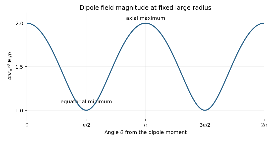
The neutral charge pair has no net electric charge, so its leading far field falls as $r^{-3}$ and depends on direction. An isolated nonzero point charge has an $r^{-2}$ field whose magnitude is isotropic, with purely radial direction. The dipole also generally has a nonzero $E_{\theta }$ component.

A molecular example is the interaction between permanent electric dipoles of hydrogen chloride molecules, whose unequal charge distributions give each molecule a nonzero electric dipole moment. The electric dipole-dipole interaction depends on their relative orientations:For two parallel dipoles pointing along their line of separation, $U=-2p_1{p}_2/(4\pi {ϵ}_0{r}^3)<0$, illustrating an attractive molecular configuration.

For an original classical calculation of the return step, neglect the residual ion's Coulomb force after release. Take a spatially uniform driving electric field $E(t)=E_0\cos \omega t$, an Electron of electric charge $-e$ and mass $m$, and zero initial position and velocity at $t_i$. With $\alpha =\omega t_i$ and $\beta =\omega t$, integrating Newton's second law givesA return requires $\beta >\alpha$ and $x(t)=0$. Define the cycle-averaged free-electron quiver kinetic energySearching the first-return solutions for release phases $0<\alpha <\pi /2$ gives a maximum near $\alpha =0.3134$ and $\beta =4.3990$, with $K_{\mathrm{return}}\simeq 3.1731U_p$. For a chosen ionization energy $I_p$, recombination into the initial state can therefore emit a photon with energy up to approximately $I_p+3.17U_p$ in this model. This is an upper return-energy scale, not a prediction of the emitted yield. It omits release probabilities, quantum interference, propagation, phase matching and depletion of the neutral gas.

The calculation explains why a long driving wavelength can increase the available return energy: at fixed $E_0$, $U_p$ grows as ${\omega }^{-2}$. It does not say that conversion efficiency improves. The Electron must return with a probability amplitude for emission that survives the microscopic dynamics and adds coherently across the gas.

An internal qubit uses two distinguishable electronic or hyperfine structure quantum states, denoted $|g⟩,|e⟩$. The ion's centre-of-mass motion has a different Hilbert space. In one approximately harmonic direction, a number state $|n⟩$ has energy $E_n=\hslash \nu (n+1/2)$, where $\nu$ denotes a motional angular frequency, not ordinary frequency. The tensor product of quantum systems gives $|g,n⟩$. Cooling towards $n=0$ prepares motion; it does not automatically prepare the internal qubit. Nor does the ground state mean a stationary point particle: zero-point energy and position spread remain.

For several ions, Coulomb forces couple their displacements into collective normal modes. Each selected normal mode has its own quantum harmonic oscillator number states, while each ion retains internal qubit states. A pulse addressing one ion can change a shared mode. This supplies a route to correlations between distant internal quantum states; it also makes residual motional excitation and unwanted excitation of other normal modes relevant. A single-ion pulse calculation alone establishes no experimental multi-ion quantum gate performance.