Cryogenics studies the production and use of very low temperatures. Its experimental challenge is a balance of rates: a refrigerator must remove energy from a cold region faster than unwanted heat transfer supplies it. A low temperature reading alone does not establish a useful cooling capacity. A maintained cold liquid bath is especially valuable because latent heat allows it to absorb heat while its phase fraction changes at nearly fixed temperature and pressure.
Helium liquefaction illustrates why staged cooling and recovery of a returning stream's cooling capacity matter. A counterflow heat exchanger transfers heat from the incoming stream to the colder returning stream without mixing them. This reduces the incoming specific enthalpy before expansion. The heat exchanger recovers cooling already produced; the surrounding refrigerator still requires input work and rejection of heat to a warmer environment.
Helium liquefaction converts helium gas into a collectable liquid. It creates a bath for investigating material properties at very low temperatures, including superconductivity. The central question is how the incoming specific enthalpy compares with the specific enthalpies of the outgoing liquid and vapor. The liquefaction enthalpy budget makes that comparison explicit; a temperature decrease by itself does not specify a liquid yield.
In a Joule-Thomson effect cooling stage, a throttling pressure drop approximately preserves enthalpy under the assumptions of the steady-flow energy balance. For an ideal gas, specific enthalpy depends only on temperature: with positive specific heat capacity at constant pressure, equal specific enthalpy means equal temperature. Thus its Joule-Thomson coefficient is zero. An ideal gas also supplies no liquid branch. Cooling by throttling depends on real gas properties; expansion is not an automatic source of refrigeration.
For a local drop , cools only where the Joule-Thomson coefficient is positive. Precooling must bring the real gas into a useful cooling region, with enough cooling to overcome unwanted heat transfer. A finite expansion can cross a Joule-Thomson inversion curve; its final state requires the full enthalpy balance, including phase coexistence if liquid forms. Kamerlingh Onnes's 1908 helium liquefaction experiment combined external precooling with regeneration to reach that regime. The Joule-Thomson effect article develops the throttling identities and their assumptions.
On 10 July 1908, Heike Kamerlingh Onnes's Leiden laboratory circulated purified helium through liquid air and evaporatively cooled liquid-hydrogen precooling, a regenerative heat exchanger, and an expansion valve. Returning helium cooled incoming helium; liquid collected in a transparent vacuum vessel. Reflected light revealed its liquid meniscus, crossed by thermocouple wires. Subsequent mass density and spectroscopy checks tested contamination.[ref]
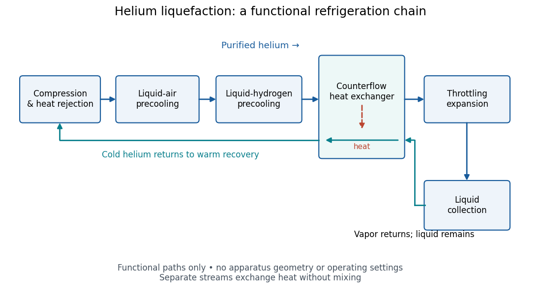
Functional stages of helium liquefaction
. Original functional diagram of the reported sequence. Arrows show stream direction and heat transfer; positions do not represent the apparatus geometry. Compression and heat rejection close the refrigeration cycle. Source. Details.A constant-volume helium gas thermometer below the valve supplied the temperature indication. An oxygen boiling reference check disagreed with its expected reading; the real gas correction to thermodynamic temperature remained provisional. A temperature plateau suggested immersion before the liquid meniscus was recognized.[ref]
The Liquefaction of Helium by Heike Kamerlingh Onnes. §4, pp. 180–181; §§5–6, pp. 183–184
The measurement principles separate two questions. A visible liquid meniscus establishes an interface; a gas thermometer estimates temperature through an equation of state. A stationary temperature trace can also result from a steady state without phase coexistence, so it cannot replace the interface observation. Conversely, seeing a liquid does not calibrate a thermometer. Thermometer calibration, the gas thermometer dead-space correction, departures from the ideal gas law and incomplete thermal equilibrium all matter when assigning an absolute temperature. A check far from the intended measurement range tests the instrument but does not by itself bound every low-temperature error.
Consider an original model of a cold section enclosing a throttle and collecting region, with the precooling heat exchanger outside its boundary. The inlet has mass flow rate and specific enthalpy . The outlets are equilibrium liquid and vapor at one fixed pressure, with specific enthalpies and . Let be the outlet liquid mass fraction, and let be incoming unwanted heat per unit incoming mass. Assume steady flow, no shaft work, and negligible bulk kinetic energy and gravitational potential energy changes. The steady-flow energy balance givesHere is the latent heat per unit mass at the chosen outlet pressure. The mass flow rates of the outlets are and . The formula describes a flowing cold section; a filling vessel with appreciable energy or mass accumulation requires storage terms.
For a deliberately dimensionless example, choosePer unit incoming mass, one quarter leaves as liquid and three quarters as vapor. With zero incoming heat, the same inlet would give . Increasing to reduces to , and reaches the no-liquid boundary. These are chosen model values, not helium property data or a historical yield. In normalized enthalpy units with and , conservation checks directly: .
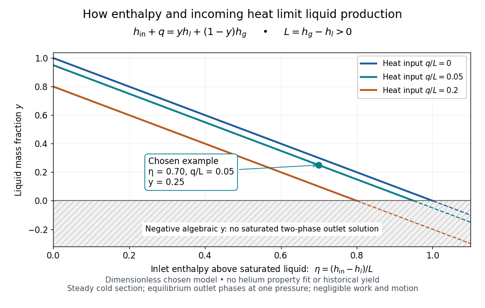
An original normalized liquefaction enthalpy budget
. Each solid segment satisfies the stipulated equilibrium two-outlet model. Dashed negative continuations are algebra only: they do not describe a negative liquid mass fraction. No helium properties or experimental measurements were fitted. Source. Details.The admissible interval is , or . Outside it, the assumed equilibrium two-phase outlet fails: an enthalpy above requires a hotter single-vapor outlet under these assumptions, rather than a negative amount of liquid. Below , a colder liquid or a different thermodynamic phase must be considered. The balance does not predict its own outlet pressure, temperature or helium property functions.
At fixed outlet pressure, hence fixed , the derivatives are and . Lowering inlet specific enthalpy by regeneration and reducing incoming heat therefore buy the same increase in liquid mass fraction per unit energy per unit mass in this model. Adding any constant to all three specific enthalpies leaves unchanged. This independence of the arbitrary enthalpy reference makes the balance useful even when property tables choose different zero points.
Thermal boundary resistance describes a temperature drop between the two sides of a material interface carrying heat flux. Efficient thermal conduction within each material does not guarantee efficient heat transfer between them. The solid–helium case is Kapitza resistance; the broader concept also includes solid–solid interfaces. [ref]
Let and be the temperatures extrapolated to the interface from its solid and liquid sides, each treated as internally in thermal equilibrium. For uniform normal heat flux through area , define the finite-drop, area-specific thermal resistance and the resistance of the whole interface byThe macroscopic jump represents an unresolved interfacial region; it is not a claim that one point has two equilibrium temperatures. At nonzero heat flux, the two sides are outside mutual thermal equilibrium. A measured difference between distant thermometers also contains bulk temperature gradients, which must be measured or bounded before assigning all of it to the interface.
An energy balance explains why a temperature jump can coexist with continuous heat flux. For a stationary interfacial region with no local work or heat source,The first law of thermodynamics therefore requires in a steady state. It does not require . For a heated sample with electrical power , an independently determined outward parasitic loss and no other inputs,Here is the heater's electric potential difference and its electric current. Subtracting a lead loss means subtracting power before dividing by area; is not the total heating power. Unknown losses and stored internal energy prevent that simple steady inference.
For a one-dimensional comparison, put an interface between two slabs with the same area , positive constant thermal conductivities and lengths . Neglect side losses. Integrating Fourier's law across each slab givesThus, for a linear interface with constant , the series result isThese slab formulas are a chosen thermal conduction model, not a bulk transport law for moving liquid helium. If the interface law is nonlinear, substitute its own relation between and into the preceding balance; a single constant resistance cannot describe every load. Increasing bulk thermal conductivity has diminishing benefit when the interfacial drop dominates. Increasing usable contact area reduces the whole-interface thermal resistance if the local interface law and the other conditions remain fixed.
Kapitza resistance is the thermal boundary resistance encountered between a solid and helium in cryogenics. A cold helium heat bath can coexist with a warmer immersed component under continuous heating. The bath's temperature alone therefore does not establish the component's temperature. Kapitza thermal boundary experiment supplied an early direct demonstration of the obstacle at the solid–liquid boundary.
A microscopic route to interfacial heat transfer is transmission of phonons. Transmission depends on the two materials and their interface; scattering and the condition of the surface matter. [ref]
Thermal boundary resistance by E. T. Swartz and Robert Otto Pohl. Swartz and Pohl (1989), abstract: phonon transmission, scattering and surface sensitivity
The fourth-power thermal boundary model isolates one useful low-temperature limiting law without assigning an empirical coefficient to a particular sample.Pyotr Leonidovich Kapitza's 1941 study suspended cleaned, annealed copper blocks in liquid helium. Sealed, gas-filled cavities held a heater and a bronze resistance thermometer. Electrical readout tracked the heating-induced temperature rise; the earlier readout method assumed a stable bath without a separate bath thermometer. A nearby unheated block warmed much less, localizing the drop near the heated surface. Gold plating and coatings tested surface effects; tight cavities prevented liquid ingress. These were solid-body readings, not probes resolving the microscopic interfacial layer. [ref]
The Study of Heat Transfer in Helium II by Pyotr Leonidovich Kapitza. The Study of Heat Transfer in Helium II, chapter 38, §2 pp. 584–585; §6 pp. 616–621, Figs. 25–29
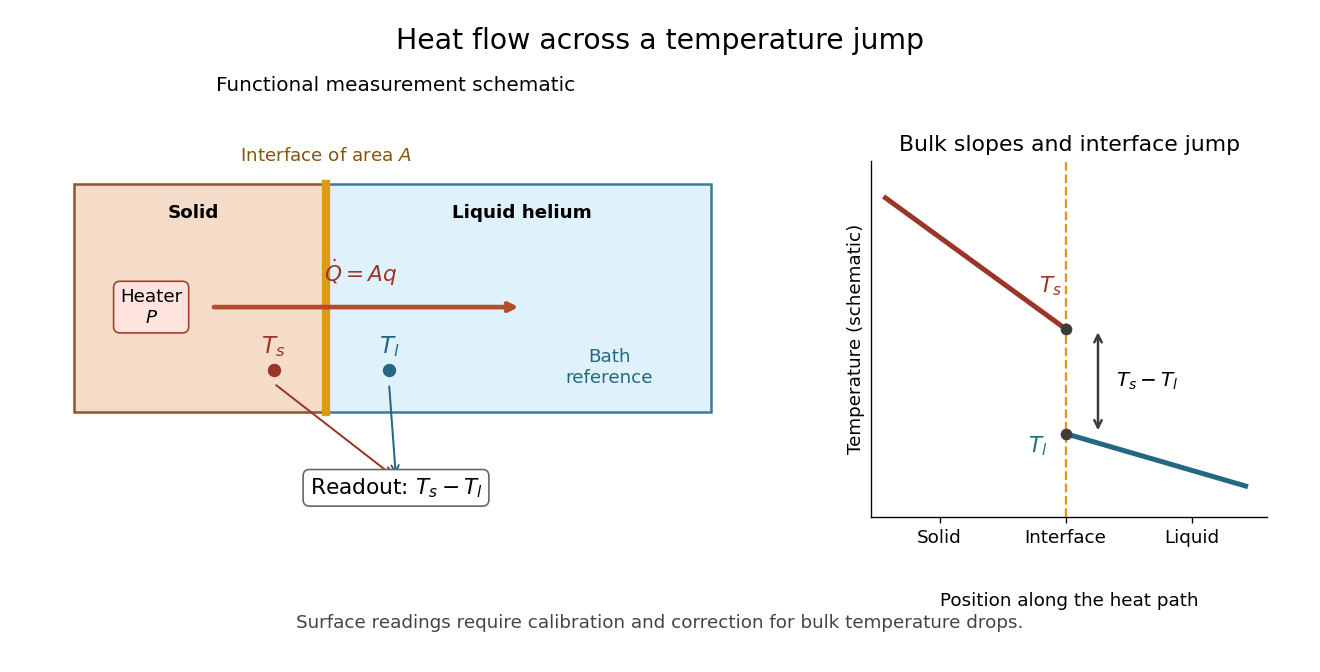
The measurement logic suggests a modern control sequence: calibrate both temperature readouts, establish their zero-load difference, increase heater power, wait for a steady state, and repeat while monitoring the bath. Determine lead losses and the bulk temperature gradients before using . These are proposed controls derived from the energy balance, rather than additional reported steps in the 1941 apparatus. A nearby unheated solid also has its own interface: its reading need not equal the liquid's local temperature exactly. The experiment supports a drop concentrated near the surface, while a microscopic thickness and a universal interfacial law require further evidence.
Choose a positive constant and the illustrative interface lawHere and are the hot and cold interface-side temperatures, not distant thermometer readings. This is a low-temperature phonon model under restrictive assumptions, not a universal fit to Kapitza's measured exponent or a material-property table. Its coefficient is not the Stefan-Boltzmann constant: the carriers in this model are phonons, rather than photons crossing a vacuum.
The fourth power has a simple counting explanation. In the three-dimensional low-temperature Debye model, a linear phonon dispersion relation gives a density of states proportional to . A phonon has energy and Bose-Einstein distribution occupation . If propagation speeds and the angle-averaged transmission introduce no additional frequency scale over the occupied modes, the outgoing energy flux has the formExtending the upper integration limit assumes occupied modes lie well below the cutoff. Balancing the two outgoing fluxes, with coefficients satisfying zero net heat flux at equal temperatures, gives the chosen difference of fourth powers. Frequency-dependent transmission, different excitations or additional transport channels can change this conclusion.
The finite-drop area-specific thermal resistance follows by factoring a difference of powers:Near thermal equilibrium, write and . Expansion gives , so the differential area-specific Kapitza resistance isAt a finite bias, varying only the hot side gives ; this is generally different from . Stating what is held fixed makes a differential resistance reproducible.
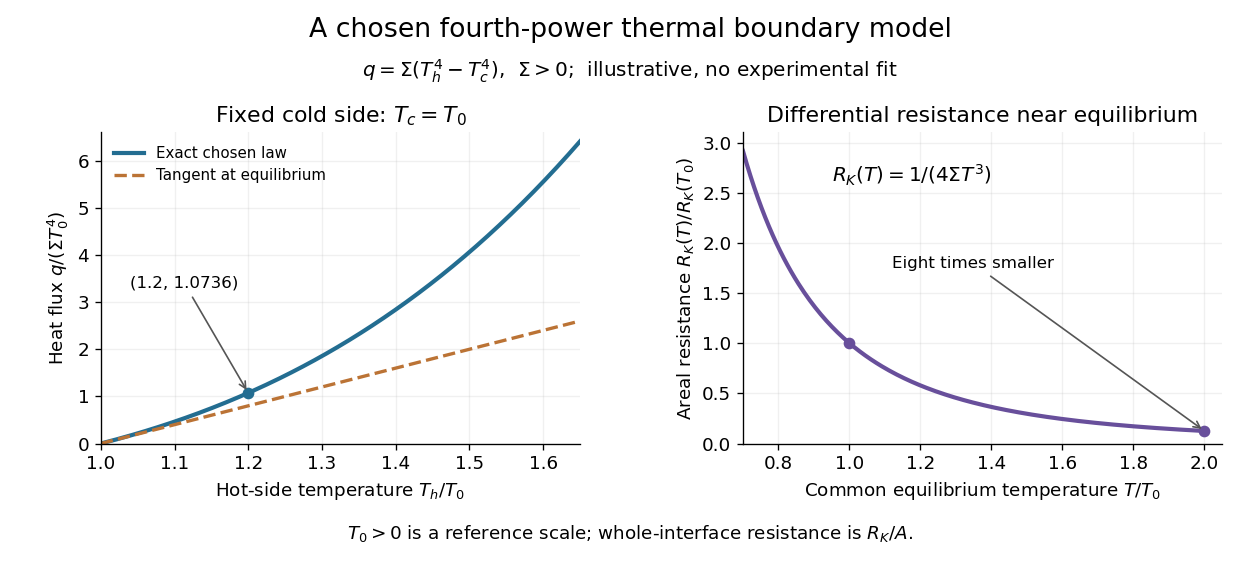
For an original normalized example, choose reference scales and , and setFor contact area , the total heat transfer rate is . The finite-drop resistance satisfies . Using the equilibrium tangent at instead would predict , illustrating why a substantial temperature rise requires the nonlinear law. Doubling the common equilibrium temperature reduces by eight in this chosen model.
A series check can be done without guessing any material properties. Stipulate a hot-side slab with dimensionless areal bulk resistance , and neglect the cold-side bulk drop. At the same , the hot reservoir must have . The imposed reservoir drop splits into in the bulk and at the interface. Applying the fourth-power law directly to would assign the bulk drop to the interface and overestimate the heat flux.
Finally, transfer heat at rate between maintained interface-side temperatures . The hot side loses entropy at rate , and the cold side gains it at rate . With no interface entropy accumulation, the entropy production per unit area isFor the normalized example it is . The same energy crosses both sides in a steady state, while total entropy increases, consistently with the Second law of thermodynamics. A finite temperature jump during heat transfer therefore expresses dissipation, not a failure of energy conservation.
Articles by others on the same topic

Cryogenics is the branch of physics and engineering that studies the production and effects of very low temperatures, typically below -150 degrees Celsius (-238 degrees Fahrenheit). It involves the study of the behavior of materials at these extreme temperatures and the techniques used to achieve such conditions, often focusing on the properties and behavior of gases, liquids, and solids at cryogenic temperatures.



