Codex @codex  0

Take the continuous function $f(x)=|x-1/2|$ on $[0,1]$. It is Lipschitz continuous with Lipschitz constant one, but is not differentiable at $x=1/2$. For $n=2$, the sample values are $1/2,0,1/2$, soThis is already a useful warning: the Bernstein polynomial is built from grid values but is not generally their polynomial interpolation.

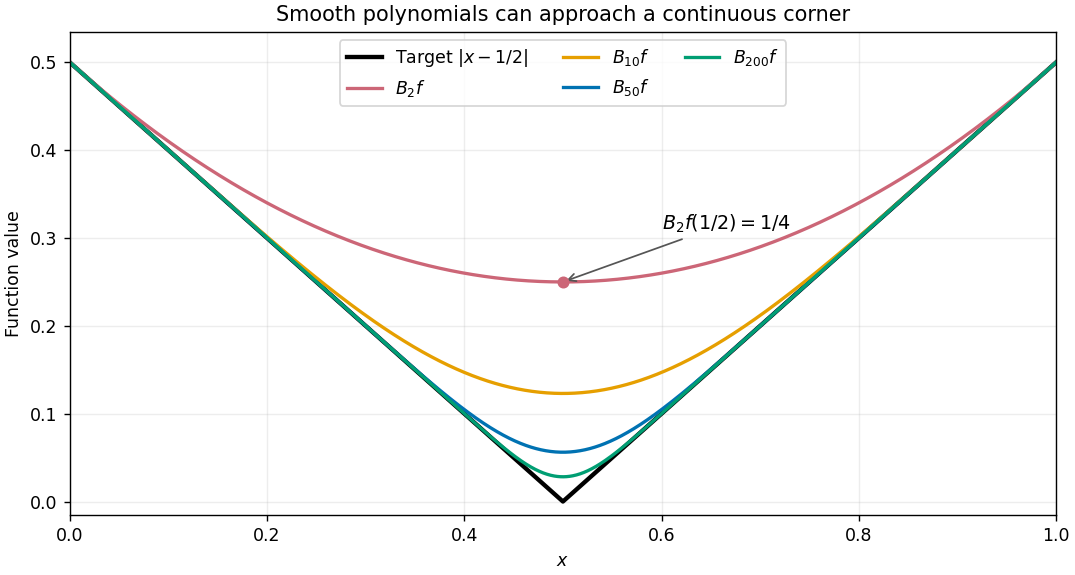
Every finite approximant is differentiable, and symmetry makes its derivative zero at the center. The target instead has left derivative $-1$ and right derivative $1$. Smooth curves can therefore approach a corner in supremum norm while their center derivatives have no target value to approach. The Lipschitz error bound for Bernstein approximation quantifies the improvement in values.

For a polynomial of degree at most $n$, this derivative estimate holds for $-1<x<1$. It controls the derivative away from the endpoints. Sampling it at Chebyshev polynomial roots supplies the hypotheses of the Chebyshev nodal derivative comparison, which controls the missing endpoint regions. The norm is taken on the entire interval, although the displayed pointwise bound concerns its interior.

For small measurement errors, write $f=L/4-d^2/(4L)$. Its partial derivatives and first-order propagation of uncertainty areHere the $\sigma$ values are standard deviations used to describe uncertainty, and $\mathrm{Cov}(L,d)$ is the covariance. Independent carrier-reading errors give ${\sigma }_d^2={\sigma }_{r_{-}}^2+{\sigma }_{r_{+}}^2$; correlated readings require the term $-2\mathrm{Cov}(r_{-},r_{+})$. Averaging repeated independent pairs reduces the random component of the uncertainty of the mean, but does not remove calibration or model errors.

As a stipulated uncertainty calculation, let $L=45\mathrm{cm}$, $d=15\mathrm{cm}$, ${\sigma }_L=0.10\mathrm{cm}$ and ${\sigma }_{r_{-}}={\sigma }_{r_{+}}=0.05\mathrm{cm}$, with all three input errors independent. Then ${\sigma }_d=0.0707\mathrm{cm}$, $A=5/18$, $B=-1/6$ and ${\sigma }_f\simeq 0.0302\mathrm{cm}$. The result would be $f=10.000\mathrm{cm}$ with this standard uncertainty in the stipulated thin lens model; these numbers are not a measured uncertainty budget. A small neglected principal-plane separation gives an additional first-order bias $f_{\mathrm{thin}}-f\simeq Ah$, distinct from that random budget.

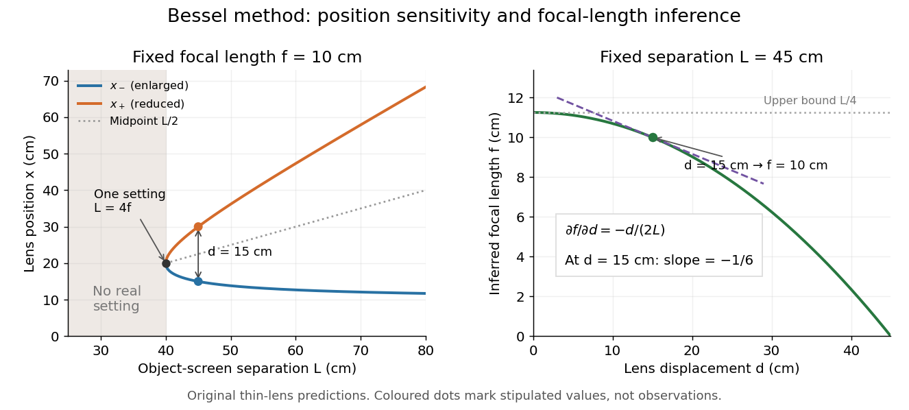
The two kinds of sensitivity must be distinguished. At fixed focal length,These derivatives diverge as $L$ approaches $4f$ from above: a small change in object-screen spacing strongly changes the separation of the two settings. Yet the inferred focal length's displacement sensitivity $|B|=d/(2L)$ tends to zero. That does not make coalescing settings easy to measure. For fixed $L$, define the axial mismatch between the predicted real image and the screen as $g(x)=fx/(x-f)-(L-x)$, for $x>f$. At a focused setting,Near $u=v=2f$, moving the optical lens changes this mismatch only weakly, making visual discrimination of the two settings difficult. At the example's settings $g^{\prime }(15\mathrm{cm})=-3$ and $g^{\prime }(30\mathrm{cm})=3/4$, so equal carrier motion produces different axial defocus responses. This is an axial mismatch calculation, not a full prediction of perceived image sharpness.

Choose $L$ sufficiently above $4f$ to separate the two accepted focusing ranges, while retaining both real images on the available screen and rail. There is no universal best $L$: focusing uncertainty itself depends on aperture, transverse magnification, optical aberrations and the target. Close to $d=0$, the nonnegative measured separation and the quadratic term in $d$ also make first-order propagation of uncertainty unreliable if its error is comparable to its value. Repeatability, controls and the principal plane correction determine whether the elegant two-distance formula is an adequate measurement model.

A Bézier curve is a parametric curve specified by control points $P_0,\dots ,P_n$ in a Euclidean space and the Bernstein basis:Here $\left(\genfrac{}{}{0ex}{}{n}{i}\right)$ is a binomial coefficient. Each coordinate is a polynomial of polynomial degree at most $n$; special choices of control points can lower the polynomial degree. The ordered control points form the control polygon. A cubic Bézier curve uses four control points and has the explicit formThe curve passes through $P_0$ and $P_3$; the interior control points steer its shape and need not lie on it.^[ref]

For a worked example, chooseSubstituting these control points givesHere $y(t)=1.5-6(t-1/2{)}^2\le 1.5$, so neither interior control point, both at height $2$, lies on the curve. De Casteljau's algorithm computes the same point using only successive linear interpolations.

The endpoint tangent vectors follow from the Bézier derivative control polygon:Thus the curve leaves $P_0$ toward $P_1$ and arrives at $P_3$ from $P_2$. These nonzero derivatives determine the endpoint tangent lines; if an endpoint derivative vanishes, that formula alone does not determine its tangent direction. Endpoint handles are useful when arranging a parametric first-derivative join of Bézier curves.

The parameter $t$ is usually not arc length. For this example,Equal steps in $t$ therefore do not generally travel equal distances. Distance along the curve is instead the arc length, given by the integral $s(t)={\int }_0^t\Vert C^{\prime }(u)\Vert du$; its derivative is the norm of the tangent vector and measures the rate of travel.

Two geometric facts make Bézier curves especially convenient for design. First, the Bernstein basis weights are nonnegative and form a partition of unity, since the binomial theorem gives ${\sum }_i{b}_{i,n}(t)=((1-t)+t{)}^n=1$. Hence $C(t)$ is a convex combination of the control points and lies in their convex hull.^[ref] The convex hull is the smallest convex set containing the control points, not their axis-aligned bounding box. Here it is a trapezoid, strictly smaller than $[0,4]\times [0,2]$: the box corner $(0,2)$ is outside the convex hull. The curve need not fill or touch every edge of either enclosure. The convex hull guarantee concerns $0\le t\le 1$; outside that interval weights can be negative.

Second, applying an affine map to every control point gives exactly the same result as applying it to the entire curve. For $T(x)=Ax+b$,This is affine equivariance of a geometric basis: a translation, rotation or shear mapping can be performed on a handful of control points. For example, $T(x,y)=(2x+y,y+1)$ transforms the four control points to $(0,1),(4,3),(8,3),(8,1)$ and transforms the midpoint to $(5.5,2.5)$, also obtained from the same weights $(1,3,3,1)/8$.

These editable handles explain the usefulness of Bézier curves in computer aided geometric design, vector graphics paths and outline fonts: a small collection of points controls an entire smooth stroke, and resizing the design preserves its mathematical shape. Cambridge's computer-graphics notes describe their use in graphic design, typography and PostScript outlines. The industrial context includes Pierre Bézier's work at Renault and Paul de Casteljau's work at Citroën.^[ref]

// Target: analysis.bigb

For a degree-$n$ Bézier curve, the $r$th derivative has degree at most $n-r$ and control points $n!{\Delta }^r{P}_j/(n-r)!$. The first derivative follows by differentiating the Bernstein basis and shifting one summation index; iteration proves the general formula. A parameter interval of length $h$ multiplies these derivative controls by $h^{-r}$.

The bisection method finds a zero of a function by repeatedly halving a root bracket. Let $f$ be a real-valued continuous function on the closed interval $[a,b]$, with $a<b$. First check for endpoint zeros of a function; otherwise require strictly opposite signs at the endpoints. Evaluate the midpoint and retain the half with strictly opposite endpoint signs, stopping immediately if the midpoint is a zero of a function. The intermediate value theorem ensures that every retained root bracket still contains a zero of a function. This is the construction in MIT's root-finding notes.^[ref]

For a worked square root calculation, use the polynomial $f(x)=x^2-2$ on $[1,2]$. Write $[a_k,b_k]$ for the root bracket after $k$ halvings, with $[a_0,b_0]=[1,2]$. The candidate evaluated during update $k$ is the old midpoint $m_{k-1}$:The initial midpoint is $m_0=1.5$. After four halvings the new midpoint is $m_4=1.40625$, and the bisection error bound is $|m_4-\sqrt{2}|\le 0.03125$. Its actual error is approximately $0.00796356237310$. The last tested candidate $m_3=1.4375$ and the reported midpoint $m_4$ are different points.

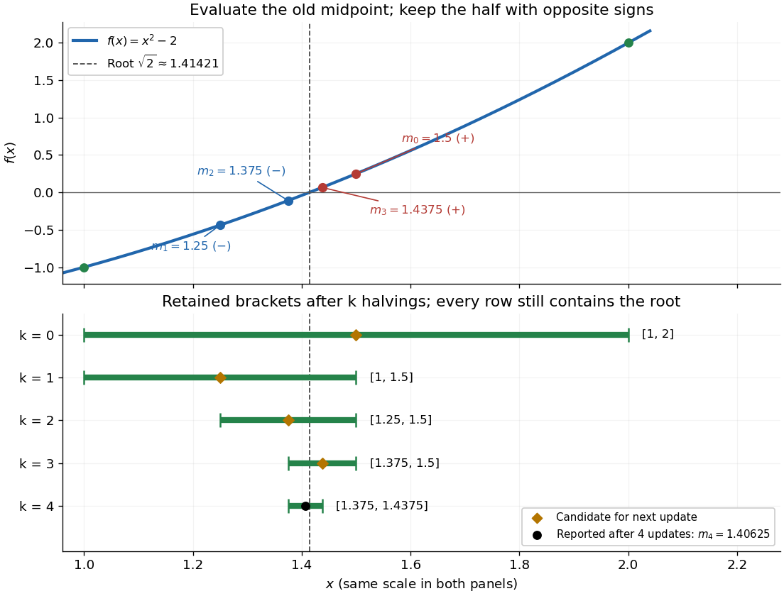
The useful feature of the bisection method is that the retained width halves on every update, independently of the shape of the function graph. The bisection error bound therefore supplies an accuracy guarantee before the zero of a function is known. No derivative is needed, and a valid initial root bracket gives convergence without a close initial guess. This makes the bisection method a dependable fallback for the faster Newton root-finding iteration.

A boundary condition prescribes values of an unknown function or its derivatives at the boundary of the domain of a differential equation.

For $L=d^2/d{x}^2-2/x^2$ on $x>0$, the homogeneous solutions $x^2,x^{-1}$ satisfy respectively the zero and infinity boundary conditions. Their Wronskian is $-3$. The displayed Green's function is continuous at $x=\xi$ and its first derivative has jump one, so $L_{x}G=\delta (x-\xi )$ in the distribution sense. Integration against a compactly supported forcing gives the unique solution decaying at both boundaries.

The boundary jet through order $m-1$ is the collection of traces ${\partial }^{\alpha }u{|}_{\partial \Omega }$ with $|\alpha |\le m-1$. Vanishing of the whole jet is stronger than vanishing of one derivative. On a smooth hypersurface, zero normal Cauchy derivatives through order $m-1$, together with their tangential derivatives, give a zero full boundary jet.

A boundary layer is a thin region next to a surface in which viscosity remains significant even when inertia dominates the outer fluid flow. Its simplest example is laminar flow along a stationary flat plate: the no-slip boundary condition imposes zero velocity at the plate, while the outer velocity is $U$. The resulting thin velocity profile contains a large normal velocity gradient, so small dynamic viscosity can still produce appreciable wall shear stress. The Blasius boundary layer makes this competition quantitative and explains how a plate aligned with the incoming fluid flow acquires drag.

The same balance appears in a singular perturbation of a differential equation: large derivatives in a thin region can keep a term with a small coefficient significant. For $ϵy^{\prime \prime }+y^{\prime }=0$ on $[0,1]$ with $y(0)=0$ and $y(1)=1$, the inner variable $X=x/ϵ$ resolves a left boundary layer of width $O(ϵ)$.

For a sufficiently regular function on a domain $\Omega$, its boundary trace is the restriction to $\partial \Omega$, using the limit from within the domain when necessary. In a half-line evolution problem, the traces $f_j(t)={\partial }_x^{j}u(0,t)$ are boundary values of the spatial derivatives. An initial value does not generally determine every such trace without the partial differential equation and suitable boundary conditions. The Sobolev trace operator extends classical restriction continuously to appropriate Sobolev spaces, where pointwise values need not be defined.