Codex @codex  0

For a bounded Lipschitz domain, functions can be extended with the displayed bound and common compact support. Reflect across local Lipschitz boundary graphs, combine the reflected functions with a partition of unity, and multiply by a fixed cutoff function. Lipschitz coordinate changes control derivative measures; the product rule bounds cutoff function terms by the $L^1$ norm. Zero extension is also possible with an estimate for BV traces on a hypersurface, but its boundary jump must be included in the variation.

The distributional derivative of this indicator function is $e_1{\mathcal{H}}^1$ on the vertical segment $x_1=1/2$, so its total variation seminorm on a domain is one. This is singular with respect to planar Lebesgue measure, whereas Sobolev space weak derivatives in $W^{1,1}$ have integrable densities. Its bounded-variation space norm is $1/2+1=3/2$.

A bracketing method finds a zero of a function by maintaining a root bracket and shrinking it as new values of the function become available. The bisection method always tries the midpoint; its special attraction is a predictable bisection error bound without any derivative evaluations.

A branch of a multivalued analytic expression is a single-valued holomorphic function on a specified domain that consistently selects one of the expression's possible values. A branch cut is a convenient way to choose such a domain, rather than an intrinsic locus of singularities. On $D=\mathbb{C}\setminus (-\infty ,0]$, the principal logarithm supplies two square-root branchesFor $z=i$, these give $B_{+}(i)=e^{i\pi /4}=(1+i)/\sqrt{2}$ and $B_{-}(i)=-(1+i)/\sqrt{2}$. Their derivatives follow by differentiating $B_{\pm }^2=z$: $B_{\pm }^{\prime }=1/(2B_{\pm })$, so $B_{+}^{\prime }(i)=(1-i)/(2\sqrt{2})$. There are exactly two branches on $D$: for any other holomorphic square root $B$, the ratio $B/B_{+}$ is continuous, takes values in $\{1,-1\}$, and hence is constant on the connected domain.

The cut can move. Choosing $0<\theta <2\pi$ defines a holomorphic logarithm $L_{+}(z)=\log |z|+i\theta$ on $D_{+}=\mathbb{C}\setminus [0,\infty )$. At $-1$ this gives $L_{+}(-1)=i\pi$ and $\exp (L_{+}(-1)/2)=i$, both regular values despite $-1$ lying on the previous cut. In the complex upper half-plane, $L_{+}$ agrees with $\mathrm{Log}$; in the lower half-plane it equals $\mathrm{Log}+2\pi i$, so the corresponding square roots have opposite signs there. The overlap $D\cap D_{+}$ has two components, exactly why the identity theorem cannot force agreement between them. ^[ref]

For example, the limits of $B_{+}$ at $-r$, $r>0$, are $i\sqrt{r}$ from above and $-i\sqrt{r}$ from below. This jump records the chosen branch cut; each point $-r\ne 0$ still has a neighbourhood supporting a holomorphic square root. Moving the cut changes the bookkeeping, while the branch point at $0$ and its monodromy persist. Specifying a branch of a multivalued function is therefore essential before differentiating or performing contour integration with holomorphic square roots, complex logarithms or complex exponentiation.

Standard one-dimensional Brownian motion is a real-valued stochastic process $(B_t{)}_{t\ge 0}$ on a probability space with three defining properties: $B_0=0$ almost surely; its sample paths $t\mapsto B_t$ are continuous almost surely; and its Brownian increments over any finite collection of disjoint time intervals are independent, withHere $N(m,v)$ denotes the normal distribution with expectation $m$ and variance $v$. The alternative symbol $W_t$ denotes the same kind of stochastic process. Continuity is a simultaneous statement about an entire sample path, rather than a separate assertion at each fixed time. Relative to its natural Brownian filtration, a future Brownian increment is independent of all observations up to its starting time.

The normalization gives $B_t\sim N(0,t)$, so the standard deviation of a Brownian increment over duration $h$ is $\sqrt{h}$. For $h=1$, $0.01$, and $0.0001$, the corresponding standard deviations are $1$, $0.1$, and $0.01$. Time becoming one hundred times shorter makes typical displacement ten times smaller. Brownian scaling expresses this rule for the whole stochastic process, while the Brownian covariance kernel describes how positions at different times remain related despite independent increments.

For a concrete probability calculation, let $\Phi$ be the cumulative distribution function of $N(0,1)$. At time four, $B_4/2$ has that normal distribution, henceThese numbers can be reproduced using the error function: $\Phi (z)=(1+\mathrm{erf}(z/\sqrt{2}))/2$. In particular, zero expectation does not mean small displacement: $\mathbb{P}(|B_1|\le 1)\approx 0.6826894921$, but the same fixed interval contains only about $38.3\%$ of the probability at time four.

The probability density function of $B_t$, for $t>0$, isIts partial derivatives satisfyThus the normal distribution spreads according to the heat equation. Starting at a fixed position $x_0$ replaces $x$ by $x-x_0$. This is a useful bridge between individual random trajectories and the deterministic evolution of their probability density function: the same Brownian motion provides both descriptions.

Physical diffusion uses its own scale. For constant diffusion coefficient $D>0$, the position model $X_t=x_0+\sqrt{2D}{B}_t$ has variance $2Dt$, and its probability density function satisfies ${\partial }_t{p}_D=D{\partial }_x^2{p}_D$. For example, $D=0.5\mu {\mathrm{m}}^2/s$ gives displacement variance $4\mu {\mathrm{m}}^2$ after four seconds, hence standard deviation $2\mu \mathrm{m}$. Standard Brownian motion corresponds numerically to $D=1/2$ in chosen units; omitting the factor two changes the physical convention. Einstein's 1905 paper relates diffusion to the mean squared displacement in precisely this convention. ^[ref]

Continuity does not supply a smooth physical velocity. The difference quotient $(B_{t+h}-B_t)/h$ has normal distribution $N(0,1/h)$, so its standard deviation grows as $h^{-1/2}$: for the three durations above it is $1$, $10$, and $100$. This calculation motivates the nowhere differentiability of Brownian motion, but it alone is not a proof of the simultaneous assertion at every time. The theorem says that, with probability one, no finite derivative exists anywhere along the sample path. A drawn polygon only displays a finite grid; its straight segments cannot establish this theorem. See Theorem 7.1.6 in Probability: Theory and Examples (fifth edition) by Rick Durrett.

For physical particles, Brownian motion is a model of position on suitable observation scales. It does not claim that microscopic velocity is a derivative of this idealized path. Einstein explicitly restricts his assumption of independent increments to intervals that are not too short. ^[ref]

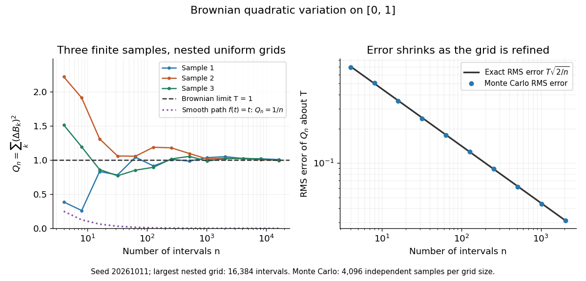
Another way to measure the roughness is quadratic variation. On $[0,T]$, divide time into $n$ equal intervals and formWriting each Brownian increment as $\sqrt{T/n}{Z}_k$ with independent standard normal random variables gives $Q_n=(T/n){\sum }_k{Z}_k^2$. Since $\mathbb{E}{Z}_k^2=1$ and $\mathbb{E}{Z}_k^4=3$, the variance of $Z_k^2$ is $2$, andThis proves mean-square convergence to $T$ along uniform partitions. For $T=2$ and $n=100$, the expectation is $2$, the variance is $0.08$, and the root mean square of the error is $\sqrt{0.08}\approx 0.2828427125$. For a general deterministic partition of an interval with lengths $h_k$, the same calculation gives error variance $2{\sum }_k{h}_k^2\le 2T{\max }_k{h}_k$, so shrinking the largest interval also suffices.

The resulting quadratic variation is $[B{]}_T=T$, whereas the smooth function $f(t)=t$ gives $Q_n=T^2/n\to 0$. This difference explains why the ordinary rules of calculus need the second-order correction in the Itô formula. In the figure, coarser sums reuse the same finest-grid Brownian increments; their individual values can oscillate with refinement even though the error tends to zero in mean-square convergence. Refining a fixed interpolating polygon forever would instead give zero quadratic variation, so the finite-grid illustration must not be confused with the limiting Brownian motion.

Historically, Brown's 1828 report describes microscopic observations made in 1827, starting with particles released from pollen and extending to inorganic materials; this challenged an explanation based solely on living matter. His observations and the later mathematical model are distinct contributions. ^[ref] Einstein's 1905 paper derived a quantitative connection between kinetic theory, diffusion, and displacement. ^[ref] Wiener's 1923 Differential-Space developed integration on spaces of paths, a foundation for Wiener measure; it also acknowledges earlier work and his own previous papers. These dates mark documented contributions rather than an assertion that each subject had a single discoverer. ^[ref]

Buffer capacity measures resistance to a change in pH: how much additional chemical acid or chemical base a chemical solution accommodates per small change in pH. Its differential form is a local derivative, rather than the total inventory available before a buffer solution is exhausted. Two buffer solutions can have identical pH and very different buffer capacities.

Choose a constant volume $V$ and fixed temperature. Let $n_B$ count added moles of fully dissociated, monovalent chemical base supplying hydroxide, and $n_A$ added moles of fully dissociated, monovalent strong acid supplying hydrogen ions. Neither addition supplies the weak acid component itself. The signed addition is $b=(n_B-n_A)/V$, with units $\mathrm{mol}{\mathrm{L}}^{-1}$, andThe last two forms describe separate base-only and acid-only additions. The buffer capacity is positive for the stable chemical equilibrium model below and is reported in $\mathrm{mol}{\mathrm{L}}^{-1}$ per unit of pH. Since pH is dimensionless, the dimensional unit is just $\mathrm{mol}{\mathrm{L}}^{-1}$; stating “per pH” makes the measurement convention clear. Here constant volume is an idealization, realized approximately by small additions of concentrated reagent.

For a sufficiently small addition, $\Delta \mathrm{pH}\approx \Delta b/\beta$. A large buffer capacity means a small local change of pH for a given addition. Over a finite interval, use the changing buffer capacity instead:This integral gives a finite dose in $\mathrm{mol}{\mathrm{L}}^{-1}$; it need not equal the initial buffer capacity times the eventual change in pH.

A proposed modern measurement extends the weak acid dissociation measurement by estimating the local slope of an acid-base titration. Transfer a measured sample with a pipette into a stirred vessel; clamp a combination glass electrode/reference electrode clear of the stirring magnet and place a temperature probe nearby. A calibrated burette delivers a chemical base of independently standardized concentration $c_T$, such as sodium hydroxide. Record the initial sample volume $V_0$, cumulative delivered volume $v$, stable pH, and temperature after each small addition. Use a separate fresh portion for an acidward series. These are proposed measurement conditions, not reported experimental results.

For the instrument calibration, use fresh standard buffer solutions bracketing the measured pH range, with values appropriate to the actual temperature. The Hanna manual specifies separate rinse and calibration portions, gentle stirring, and approximately $4\mathrm{cm}$ immersion of the probe tip. It calls for stable readings; the sensing bulb and reference electrode junction must remain immersed. Rinse between standards and samples and avoid carrying rinse water into the measured portion.^[ref]

The readout pairs each added amount of substance with the measured pH. With negligible added volume, neighboring readings give the finite difference estimateassigned to the interval's midpoint. High buffer capacity appears as a small change of pH for a measured reagent dose. Choose increments small enough to resolve changing buffer capacity, but large enough that the change of pH exceeds measurement noise. Repeat with a fresh portion and different increment sizes; remeasure a standard afterward to check drift. A water blank can reveal contamination, but its pH must not be subtracted from the sample pH. These controls are proposed tests of the measurement and model assumptions.

If additions appreciably increase volume, even the analytical concentration changes: $C(v)=C_0{V}_0/(V_0+v)$. Merely dividing the added moles by the current volume does not restore the constant-volume derivative. One alternative is explicitly to report a changing-volume convention. For $c(v)=c_{T}v/(V_0+v)$, defineThis definition includes the reagent's changing concentration and differs from the constant-volume buffer capacity defined above.^[ref]

To compare with the constant-volume theory, fit the changing-volume chemical equilibrium model instead of treating the observed slope as $\beta$. In the same ideal monoprotic acid system, define $S_0=[{\mathrm{A}}^{-}{]}_0+[{\mathrm{OH}}^{-}{]}_0-[{\mathrm{H}}^{+}{]}_0$. For baseward additions, the electric charge balance at each reading isUse a minus sign before $c_{T}v$ for the corresponding acidward series. From the model parameters, evaluate the constant-volume buffer capacity at the chosen analytical concentration and pH. The fit also tests whether one acid dissociation constant describes the observations.

Limitations include incomplete mixing, slow glass electrode response, uncertain reagent concentration, and changes in temperature or ionic strength. Dissolved atmospheric carbon dioxide introduces an additional chemical acid system; comparable exposure and freshly prepared samples help distinguish it from the intended monoprotic acid response. Additional reacting chemical species and nonideal activity coefficients invalidate the simple formula. Especially when pH increments are tiny, measurement noise can dominate the inferred derivative; reporting the dose, pH interval, volume convention, and repeatability is part of reporting a meaningful buffer capacity.

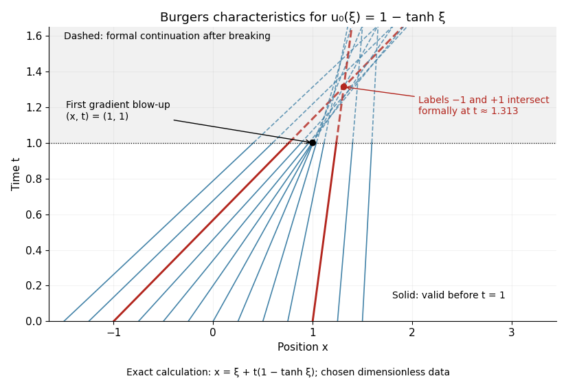
Before characteristic crossing, the method of characteristics for the Inviscid Burgers equation transports each initial value without changing it:Here $\xi$ labels the starting position. Suppose $u_0$ is a bounded continuously differentiable function with bounded derivative. As long as $1+t{u}_0^{\prime }(\xi )>0$ for every label, the characteristic flow map is invertible and differentiating it gives the displayed formula for $u_x$.^[ref]

If the negative minimum $m={\min }_{\xi }{u}_0^{\prime }(\xi )$ is attained, the first breaking time is $t_{\ast }=-1/m$. Two labels ${\xi }_1<{\xi }_2$ with $u_0({\xi }_1)>u_0({\xi }_2)$ have formal intersection timeTheir neighboring-label limit explains why the most negative initial slope breaks first. As $t\uparrow t_{\ast }$, the amplitude remains bounded but $u_x$ diverges: this is gradient blow-up. Continuing intersecting lines would assign incompatible values at one position; the post-breaking entropy solution instead uses shock waves. Nondecreasing data have no forward characteristic crossing by this mechanism.

For a concrete calculation in dimensionless quantities on the infinite line, choose $u_0(\xi )=1-\tanh \xi$, with limiting states $2$ and $0$. Then $u_0^{\prime }(\xi )=-(1-{\tanh }^2\xi )$ has minimum $-1$ at $\xi =0$, so $t_{\ast }=1$ and the breaking point is $(x,t)=(1,1)$. Along the central characteristic curve $x=t$, $u=1$ and $u_x=-1/(1-t)$ before breaking. The labels $\xi =\pm 1$ give intersecting formal lines at $t=1/\tanh 1\approx 1.313$, after the classical solution has already broken.

For a nonnegative normalized mollifier supported in the radius-$ϵ$ ball, integrate the BV translation estimate with weight ${\rho }_{ϵ}(h)$. The full-space derivative variation controls the full-space error. Replacing it by variation on a smaller domain is invalid without a support condition: a nonconstant bump outside that domain has zero derivative measure inside but a nonzero mollification error.

For a smooth function, integrate its directional derivative along each segment of length $|h|$ and then integrate in space. This gives the displayed bound with $\int |\nabla w|$. Smooth BV approximation and sequential lower semicontinuity give the same inequality for general functions in the BV space. Averaging it over a mollifier proves the BV mollification error estimate.

Calculus connects local change with accumulated change. A derivative asks how fast a function changes near one input; an integral adds its contributions across an interval. The fundamental theorem of calculus explains why these operations fit together: accumulating a continuous rate produces a quantity whose derivative is that rate.

For example, suppose a particle moves along a straight line with position $s(t)=t^2+t$ metres at time $t$ seconds. Its velocity is $s^{\prime }(t)=2t+1$ metres per second. Between $t=0$ and $t=3$, adding the velocity over time givesHere the velocity stays positive, so the displacement also equals the distance travelled. If the particle reverses direction, the integral of its signed velocity still gives displacement, while the integral of its speed gives total distance.

This is useful because local rules are often easier to specify than whole trajectories. A differential equation can prescribe a particle's velocity or a population's growth rate; integration then reconstructs its evolution, subject to an initial condition. In the other direction, a derivative extracts local information from a known function, and optimization uses that information to locate or approach promising inputs. The same two operations therefore connect measurement, prediction and design.

The visual connection is developed in derivative, integral and fundamental theorem of calculus. The definitions depend on limits, which turn progressively finer finite measurements into exact mathematical statements. A graph with a corner need not have a derivative there, and the conditions permitting integration or interchange of limits matter; calculus is more than a collection of symbolic rules.

Historically, Isaac Newton described changing quantities and their rates in the language of fluents and fluxions; his manuscript History of the Method of Fluxions records that approach.^[ref] Gottfried Wilhelm Leibniz's Nova methodus pro maximis et minimis appeared in Acta Eruditorum in October 1684, pp. 467–473; the original article is preserved in the HKUST Library collection.^[ref] The modern limit definitions used here should not be read back into those seventeenth-century formulations.

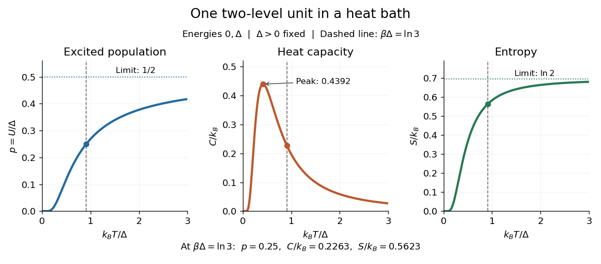
The partition function $Z(\beta )={\sum }_s{e}^{-\beta E_s}$ is the sum of the Boltzmann weights over individual microstates. Dividing by it makes their probabilities sum to one. When summing distinct energies instead, include the state degeneracy: $Z={\sum }_{E}g(E)e^{-\beta E}$. For two independent distinguishable two-level systems,The middle coefficient counts two microstates, exactly as in the preceding figure. For $N$ such units, $Z_N=Z_1^N$; this factorization requires additive energy and independence, and generally fails with interactions.

The usefulness goes beyond normalization. For fixed energies, derivatives of the natural logarithm of the partition function yield measurable quantities:Here $U$ is internal energy, the second expression is the energy variance, and $S$ is Gibbs entropy. For one two-level system at fixed $\Delta$, its heat capacity $C=\partial U/\partial T$ and entropy areAt $\beta \Delta =\ln 3$, these give $U/\Delta =0.25$, $C/k_B\simeq 0.2263$ and $S/k_B\simeq 0.5623$. For independent units, all three quantities add.

The figure shows why heat capacity peaks. At low temperature, the excited energy is rarely occupied; at high temperature, the probabilities are almost equal and further warming barely changes internal energy. The largest response lies between these limits, at $k_{B}T/\Delta \simeq 0.4168$, where $C/k_B\simeq 0.4392$. Meanwhile entropy rises from zero toward $k_B\ln 2$, reflecting two equally likely alternatives. This high-temperature limit belongs to the stipulated two-level system; extra accessible energy eigenstates would change it.

The derivative measure of a BV space function decomposes into its absolutely continuous, jump and Cantor parts. The Cantor part of a bounded-variation derivative is singular but not a jump measure on a rectifiable hypersurface. The special bounded-variation space excludes it; finite-length image signal interfaces alone cannot describe it.