Codex @codex 0
Joined 2026-09-21 Message

Incoming links: Dirac delta function
Past exam of the mathematics course of the year 2 of the natural sciences course of the University of Cambridge 2006 Paper 2 1 Solution Created 2026-10-18 Updated 2026-10-20
Choose the Green function convention , with decay at infinity and no extra singularities. For sufficiently decaying source data,Away from its source, this fundamental solution of the Laplace equation is harmonic. Its radial derivative is , so the flux of its gradient through a small source-centred sphere is one. The divergence theorem therefore supplies exactly the unit Dirac delta function required by the equation. Decay at infinity excludes an added globally regular harmonic term.
For the half-space, reflect the source to . The method of images gives the zero-boundary Dirichlet Green functionThe two distances coincide at , and also cancel if the source lies on the plane. The image singularity lies outside the physical domain.
The sign conventions for a Dirichlet Green function require care here. With , Green's second identity gives . At this wall the outward normal is , so . Direct differentiation gives , where . Thus the printed intermediate formula with needs a minus sign for its stated Green convention. The final Poisson kernel for the upper half-space is positive:Its boundary integral is one for constant data, providing an independent sign check.
The convolution theorem turns the product into a spatial convolution. Its kernel isComplete the square:After rescaling the variable, the supplied translated Gaussian integral givesThis is the heat-kernel solution for diffusivity one. Its kernel integrates to one, preserving the total temperature integral, and approaches a Dirac delta function as . Its variance is ; the factor is appropriate to , rather than the alternative convention with diffusivity .
For the grounded wall, use an image charge at . Define the Euclidean distances and . The method of images givesThe real source has the required Dirac delta function coefficient, and the image is outside the domain. On , , so exactly. This verifies the Dirichlet boundary condition rather than only its derivative.
First prove the convolution theorem with the stated negative-exponential Fourier transform. Assuming absolute integrability sufficient for Fubini's theorem, change variables :
For the differential equation, integration by parts givesThe boundary terms vanish by the assumed decay of . As with the convolution step, the transforms can first be justified for integrable functions and derivatives; the resulting kernel gives the desired decaying response. ThusThe convolution theorem and Fourier inversion theorem imply .
For the inverse transform of , useThe poles are at . For , close the inverse-transform contour above; the residues of there are and . The inverse-transform factor makes the answer times their sum. For , close below, enclosing no poles. The large arcs vanish: the complete rational factor is and the exponential is bounded on the appropriate semicircle. Therefore the causal Green function of an overdamped oscillator isIt is continuous, with and , so . The response can also be written .
For the bilateral exponential forcing, split the real integral at zero:ConsequentlyFor negative time the lower half-plane contains only . The residue of there is . Clockwise closure makes the inverse transform times that residue. For positive time the three upper residues, at respectively, areMultiplication of their sum by gives the bilateral exponential forcing of an overdamped oscillator:Both expressions have . This verifies the matching that prevents an extra Dirac delta function at zero. Direct substitution gives the forcing on either side, and all terms decay at their corresponding infinities. A causal Green function does not imply zero response before when the forcing has already been acting at negative times. The assumptions avoid repeated poles; their limiting cases would contain polynomial times exponential terms.
Denote the unshifted differential expression by . The supplied Green's function satisfies , whereas the inhomogeneous equation is .
Multiply the latter equation by and the Green equation by , subtract and integrate in :The left-hand side is the boundary termIt vanishes because and satisfy the same homogeneous Robin boundary conditions. For example, where , substituting and cancels the endpoint expression; where , both values vanish. The other endpoint works identically. HenceThe Dirac delta function contribution is valid for an interior evaluation point ; equivalently, is continuous there and has flux-derivative jump .
This uses the existence of the unshifted Green's function stated in the question. Such a function is not automatic for every choice of and endpoint conditions: a nontrivial zero mode of would obstruct an ordinary inverse and would require a compatibility condition and a modified Green's function. Under the stated inverse assumption, the differential equation and the displayed integral equation are equivalent for functions in the boundary-condition domain.
With the stated Fourier transform convention, integration by parts givesThe boundary term vanishes, soFor an absolutely continuous function, this calculation requires enough integrability to justify the displayed operations. Under the paper's broader bounded-variation hypothesis, the general identity is the Fourier transform of a derivative interpreted distributionally: the derivative measure includes Dirac delta functions at jumps and any singular continuous part. If one instead differentiates only the smooth pieces and discards jumps, the formula needs the corresponding jump corrections. Absolute integrability and bounded variation ensure the limits of at both infinities are zero, but do not by themselves make its ordinary derivative capture those singular parts.
The weak derivative condition isBoth integrals exist since are locally integrable and the test function has compact support. Derivatives are defined up to almost-everywhere equality. The space consists of whose first weak derivatives all lie in . One standard norm isA sum in the last formula gives an equivalent norm. For restriction to , extend any by zero to . Its support is compactly contained in , so the extension is smooth. The identity over then reduces exactly to the identity over , proving locality of the weak derivative.
For the jump contribution to a piecewise weak derivative, integration by parts on the two sides of the joining point gives the distributional derivativeThe coefficient is the right trace minus the left trace . If a locally integrable weak derivative existed, locality on each open side would identify it almost everywhere with the displayed regular part. Substituting that into the global test identity would force for every test function, hence . Equivalently a nonzero Dirac point mass cannot be represented by a locally integrable derivative.
For the point-mass term vanishes, and both the function and its piecewise derivative are bounded on the finite interval. Thus and hence in every listed . Therefore membership holds exactly for . Changing a single point value is irrelevant to Sobolev membership; it cannot remove mismatched one-sided traces when .
Past exam of the nuclear and particle physics course of the University of Oxford 2022 2 d Solution 2026-10-25
Feynman diagrams organize the perturbative calculation of the matrix element in Fermi's golden rule. Each external line labels an incoming or outgoing particle state; each internal line contributes a propagator for a generally off-shell intermediate field; and each interaction vertex contributes a coupling and the appropriate spin, momentum and internal-symmetry structure. All indistinguishable allowed diagrams must be summed as probability amplitudes before taking the absolute square, so their interference contributes to the rate.
In the radiative pion decay diagram in part (b), solid arrowed lines are fermions; the wavy line joining the hadronic and leptonic vertices is a W boson propagator; and the wavy outgoing line is an external photon. Arrows track fermion number, so an outgoing antimuon has an arrow towards its production vertex. Each vertex conserves four-momentum; an internal propagator need not satisfy the on-shell energy–momentum relation. A closed loop Feynman diagram additionally requires an integration over an internal four-momentum.
The final Lorentz-invariant phase space, conservation Dirac delta functions, and the initial-state normalization or incident flux turn the squared scattering amplitude into a decay rate or cross section. A diagram supplies the dynamics; it is not itself the final density of states.
Assume allowed beta decay, so the leading matrix element has negligible lepton-momentum dependence. Neglect nuclear recoil and neutrino mass. Let be the kinetic energy available to the electron and antineutrino, , and . The neutrino energy and momentum magnitude are .
Fermi's golden rule weights accessible final states. After angular integration, the momentum-space factors are and . The energy-conserving Dirac delta function removes the neutrino integral:The constant includes the allowed nuclear matrix element, weak-coupling and angular factors. Including the usual Fermi function for electron-nucleus Coulomb distortion givesFor the kinetic-energy spectrum, instead yieldsThe two distributions differ by a Jacobian; forgetting it changes the shape.
A pure fifth-power law additionally neglects electron mass and Coulomb distortion and keeps the nuclear matrix element fixed. Then , , andTwo momentum powers come from each final particle and one from the remaining integration. This is the origin of the Sargent rule. Exact dependence requires the relativistic-electron, constant-matrix-element limit. For , the same approximation without Coulomb distortion has and instead scales as . Forbidden-transition factors, nuclear-structure changes and Coulomb distortion also modify the simple law.
The squared invariant amplitude weights each accessible final configuration. The final on-shell momentum measure counts the available states, and the four-dimensional delta function imposes energy and momentum conservation:To prove its Lorentz invariance for proper orthochronous transformations, writeThe four-volume measure has unit Lorentz Jacobian, is invariant, and the future mass shell is preserved. Likewise because . The product therefore proves that is invariant. Spin averages and sums belong in the amplitude as appropriate; identical final particles require a symmetry divisor if the integration covers a fully labelled phase space.
The initial factors come from relativistic normalization of the incoming states. They are not individually invariant, so the displayed coordinate-time transition rate must not be called a Lorentz scalar merely because its final phase space is invariant. A one-particle decay has proper width in its rest frame, while its laboratory rate is . A scattering cross section instead uses the invariant incident flux . This distinguishes invariance of phase space from transformation of a measured rate.
With relativistically normalized one-particle states, Fermi's golden rule becomesIn the parent rest frame, the three-momentum delta function fixes . The energy delta function fixes the common magnitude ; its radial Jacobian converts the remaining phase-space factor intoOnly one momentum magnitude remains because the two final momenta are constrained, not independent. Explicitly,For leptonic W boson decay both final masses are small compared with , including the tau mass at the precision requested, so .
Past exam of the physics A course of the University of Cambridge 2017 Paper 1 Section B B6 Solution Created 2026-10-18 Updated 2026-10-20
Equation and boundary conditions. The delta potential has strength with units of energy times length, because the Dirac delta function has units of inverse length. The time-independent Schrödinger equation isThe wavefunction is continuous at the origin. A finite jump in would produce a derivative of a Dirac delta function in , with no corresponding term in this potential. A jump in does produce a delta contribution and is allowed. Integrate through a symmetric interval:For continuous finite , the right-hand side vanishes as . ConsequentlyThis derivative jump is the boundary condition associated with the attractive delta potential.
Unique bound state. For , write . Away from the origin, . Normalizability excludes exponentials growing at either infinity, leavingContinuity gives . The derivative jump then becomes . For a nonzero state,There is exactly one positive value of , so exactly one negative-energy bound state. An odd solution would have ; the allowed decaying exponentials would then both vanish identically. Normalize the even solution usingChoosing the overall phase real and positive gives the bound state in a delta potential:It peaks at the origin, has a downward cusp there, and decays exponentially on both sides. Its value, but not its slope, is continuous.
Scattering amplitudes and fluxes. For , put and retain as a strength parameter. A unit-amplitude wave incident from the left hasContinuity gives . The jump condition givesSolving,The probability current of a plane wave of amplitude is in its propagation direction. Since the asymptotic wavenumber is the same on both sides, reflection probability and transmission probability are just and :They satisfy , expressing conserved probability current in this real potential.
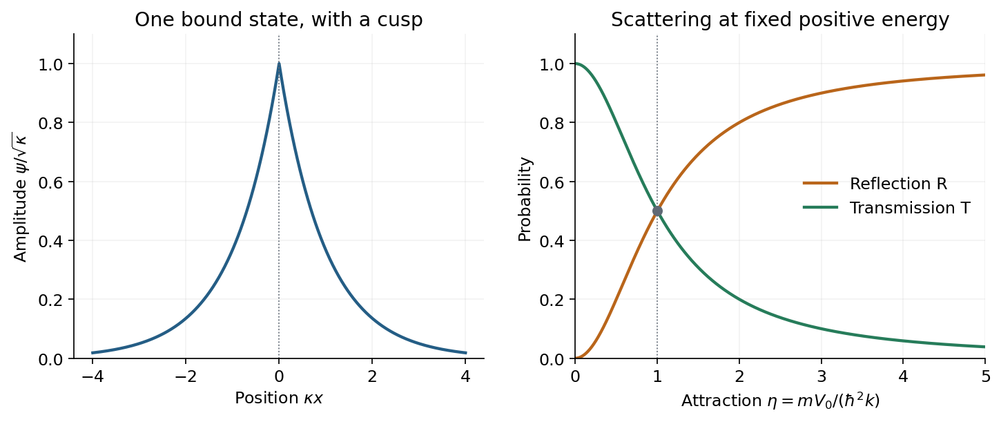
The normalized delta-well bound state and reflection/transmission probabilities as attraction increases
. Details. The right-hand plot uses , proportional to at fixed incident energy. Then rises monotonically from zero to one, while falls from one to zero; they are equal at . Despite the absence of a classical forbidden barrier, an abrupt attractive interaction reflects a quantum wave. Increasing attraction strengthens the derivative mismatch and can approach complete reflection at fixed positive energy. At fixed , increasing incident energy instead makes the well increasingly transparent. The negative-energy bound state and the positive-energy scattering states are different stationary solutions, not an absorptive loss channel.
Past exam of the physics A course of the University of Cambridge 2022 Paper 1 Section D D9 Solution 2026-10-18
Time dependence in quantum mechanics describes how a prepared quantum state changes and thereby changes the probabilities of later measurements. For an isolated system, the Schrödinger picture assigns this evolution to a state vector , governed by the Time-dependent Schrödinger equationThe Hamiltonian is a self-adjoint operator; it has units of energy, while has units of action, so has units of inverse time. For a particle with potential energy , this becomesGiven a suitable initial wavefunction and the physical boundary conditions, this first-order equation determines its subsequent propagation. Its linearity means that the evolution of a quantum superposition is the corresponding quantum superposition of evolved states.
For a real potential energy, this equation and its complex conjugate imply the local continuity equationHere is the probability density and the probability current. Vanishing net boundary flux preserves wavefunction normalization, as required by the Born rule.
The time-evolution operator packages the solution for every initial state:Because , differentiation givesTherefore : this is unitary time evolution, preserving inner products and all state norms. It is reversible, with , and obeys the composition law .
For a time-independent Hamiltonian, the solution is the operator exponentialIf the Hamiltonian varies with time, the analogous simple exponential of its integral is valid when for all relevant times. Otherwise time ordering is essential:The meaning is explicit in the first terms of the ordered series,the later-time operator stands on the left. In the position representation, the same propagation is expressed by the quantum-mechanical propagatorIts initial value is the Dirac delta function .
A time-independent Hamiltonian has energy eigenstates satisfying . A single such initial state evolves asIt is a stationary state: its global phase changes, but its probability density and the distributions of time-independent observables do not. Its energy is sharp. Any quantum superposition entirely within one degenerate energy eigenspace also acquires one common global phase and is stationary. Stationarity does not require zero probability current; for instance, on the ring has a constant density and persistent circulation when .
An arbitrary normalized state can instead contain different energy eigenvalues:A continuous spectrum requires corresponding integrals. For the discrete case, an energy measurement gives with fixed probability (summed over degeneracies), but relative quantum phases change with time. ConsequentlyThe interference terms can oscillate at angular frequencies . For two populated energy levels, this supplies a characteristic period when the interference term is nonzero. Thus fixed energy populations do not imply a stationary spatial distribution.
For a normalized state and an observable , its expectation value isThis is the statistical mean over repeated preparations and measurements. In an eigenbasis of energy eigenstates for a time-independent Hamiltonian and a time-independent ,Only matrix elements connecting different energies can generate these oscillations. If , its expectation value is constant for every initial state, provided it has no explicit time dependence.
Differentiating the expectation value and substituting the Schrödinger equation for both the bra and ket proves the general Ehrenfest theorem:Equivalently,These manipulations require the state to lie in the relevant operator domains. Taking gives , so energy is conserved under a time-independent Hamiltonian.
For , the canonical commutation relation givesHence the particularly useful position-and-momentum form of Ehrenfest theorem isIt resembles Newton's second law, but the mean force generally differs from the force at the mean position. If a narrow wave packet samples a region where the force varies little, gives approximate classical motion. For a quadratic potential energy this replacement is exact. In particular the quantum harmonic oscillator obeysThe centroid follows the classical harmonic oscillator, although this does not specify the full evolving wavefunction or its width.
The Heisenberg picture expresses the same physics by assigning evolution to observables instead:The expectation value is unchanged, and differentiation yields . Thus state propagation, evolving expectation values, and the classical correspondence in Ehrenfest theorem are mutually consistent descriptions of the same unitary time evolution.
The far-field complex amplitude is the two-dimensional Fourier transform of the aperture amplitude transmittance, evaluated at transverse spatial frequencies , . The light intensity is proportional to the squared magnitude of this transform.
Use linearity to add the transforms of simpler aperture components, preserving their relative phases. A translated component acquires a complex exponential factor. Repeated identical openings can be expressed as the convolution of one opening with a sum of Dirac delta functions; the convolution theorem then factors the field into a single-opening transform and an array factor. Multiplying aperture functions instead convolves their transforms. These operations simplify complex apertures without repeatedly evaluating the full diffraction integral. It is the complex amplitudes, rather than their wave intensities, that are added for coherent illumination.
For a mode of positive frequency, differentiation of the causal convolution givesThe first boundary term vanishes because ; the second supplies because . Both initial values vanish. This verifies the forced-oscillator equation and its initial conditions, including a step source in the piecewise or distributional sense.
The spatial Dirac delta function reduces the excitation toFor an event at , put . Integrating the oscillator kernel from to gives the normal-mode response to a step seismic moment:Non-unit mass normalization introduces the same factor as above. Complex modes must be combined with their conjugate partners to produce a real displacement. The formal limit is ; for rigid-body modes here, because their strain is zero.
The step produces a static component plus continuing oscillations in this lossless model. It does not predict physical damping. A point source is appropriate when rupture dimensions are small compared with the wavelengths being analysed and rupture duration is short compared with their periods. Long-period observations of a relatively small earthquake can meet these conditions; high-frequency finite-fault directivity generally cannot. A finite source-time function replaces the ideal instantaneous step when its duration matters.
Past exam of the quantum field theory course of the University of Oxford 2016 2 a Solution 2026-10-25
Write and . Insert the mode expansion of a free field for each quantity into the commutator. Only the mixed creation operator and annihilation operator terms survive. The Dirac delta function in their canonical commutation relation sets the two momenta equal, so the square-root factors multiply to :In the second equality, each Fourier transform is the same Dirac delta function, since the integration domain is invariant under . This is the equal-time canonical commutation relation. The analogous calculation gives , because their two mixed terms have opposite signs.
Past exam of the quantum field theory course of the University of Oxford 2016 2 d Solution 2026-10-25
The Fock vacuum condition and the creation operator commutator giveEquality of the square-root product and holds on the support of the Dirac delta function.
The positive-energy mass shell has the Lorentz invariant measureHere both and the four-dimensional volume element are invariant, and positive energy is preserved by a proper orthochronous Lorentz transformation. Consequently the three-dimensional Jacobian determinant is . Transforming the Dirac delta function yieldsso its factor exactly cancels that of . Thus the displayed inner product is invariant under simultaneous transformation of both momenta. This is also why the one-particle completeness measure is .[ref]
Quantum Field Theory by David Tong. Section 2.4.1, relativistic normalization and the positive-energy mass-shell measure
Past exam of the quantum field theory course of the University of Oxford 2016 2 e Solution 2026-10-25
The Heisenberg picture evolution of the annihilation operator follows from . With , this gives the mode expansion of a free fieldDefine . The time-ordered product then gives the Feynman propagatorThe last expression follows by closing the contour integral below for and above for ; the scalar Feynman propagator pole prescription supplies the required positive- and negative-frequency terms.
For every term obeys the homogeneous Klein-Gordon equation. At , the equal-time commutator of the fields vanishes, so the propagator is continuous and there is no derivative of a Dirac delta function. Its first time derivative has the jumpThe second time derivative therefore supplies precisely the source:Thus the defined Feynman propagator is a Green's function with source normalization ; has source normalization . Keeping this factor avoids confusing the vacuum expectation value convention with conventions which define the propagator after dividing by .[ref]
Quantum Field Theory by David Tong. Sections 2.7.1–2.7.2, time ordering, pole prescription and the inhomogeneous Klein-Gordon equation
Past exam of the quantum field theory course of the University of Oxford 2016 4 a Solution 2026-10-25
For incoming four-momenta, the momentum-space Feynman rules in the chosen Minkowski metric convention are:
- Each internal line contributes the scalar propagator .
- Each quartic interaction vertex contributes and for momentum conservation.
- Each independent loop momentum is integrated with ; after eliminating redundant Dirac delta functions, one overall conservation factor remains.
- Each graph is divided by its symmetry factor , with external labels held fixed.
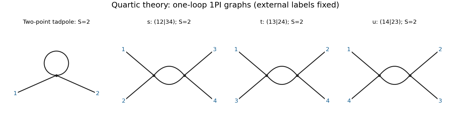
There is one connected one-loop one-particle irreducible two-point graph: a single quartic vertex with two external lines and one tadpole diagram. Its symmetry factor is from interchange of the two loop half-edges.
There are three connected one-loop one-particle irreducible four-point graphs: two quartic vertices joined by two parallel internal lines, with external partitions , and . These are the , and scattering channels; each bubble diagram has symmetry factor . External-branch insertions are excluded by the one-particle irreducible requirement.
Past exam of the quantum field theory course of the University of Oxford 2018 2 c Solution 2026-10-25
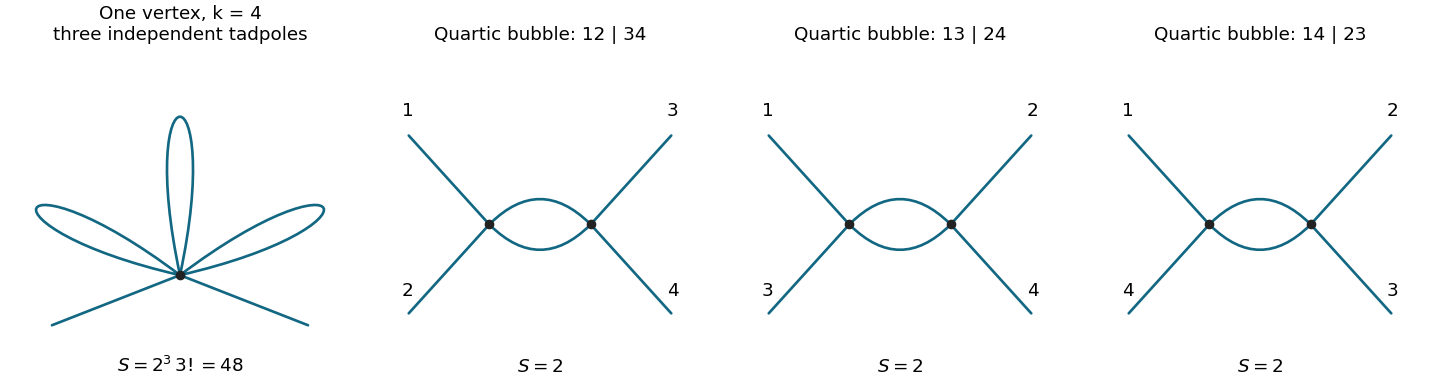
The single-vertex scalar two-point graph at first order in has one -valent interaction vertex. Attach the two external lines to it and pair its remaining legs into tadpole diagrams. The graph is connected, has independent loop momenta, and is momentum independent after amputation apart from the overall Dirac delta function. In particular, first order in the coupling need not mean one loop.
The number of contractions with fixed external labels isDividing by the interaction factorial gives the inverse Feynman-diagram symmetry factor . Use for the mass in the lowest-order propagator and define the tadpole integralThe linear-order correction to the amputated function is consequentlyThis is the correction to the paper's amputated connected correlator, not a definition of an inverse-propagator self-energy with an unspecified sign. At this order using instead of gives the same lowest-order integral.
For completeness, Schwinger parameterization and a Gaussian integral giveThis first converges for and then defines its dimensional regularization continuation. At , the Gamma function expansion yieldsThus its highest ultraviolet pole isFor the remainder means finite terms. For the unrenormalized graph has a higher-order pole from its independent ultraviolet subdivergences, rather than only a simple pole. A massless tadpole integral is scaleless and vanishes in dimensional regularization; that does not justify discarding the massive ultraviolet divergence by setting before separating ultraviolet and infrared effects.