The Doppler effect is a change between emitted and received frequency caused by motion of the source or receiver. An approaching siren can send more wave crests per second to a microphone than the source emits per second; a receding siren sends fewer. The source need not change its own oscillation. The Doppler shift is , where is emitted frequency and is received frequency, both measured in hertz.
For acoustic waves, motion must be specified relative to the material carrying the wave. The speed of sound is measured in that material's rest reference frame. Moving the source changes the spacing of successive wavefronts; moving the receiver changes how quickly it crosses those wavefronts. These two mechanisms give different exact factors in the classical Doppler effect for sound, even for the same closing relative velocity.
This makes a microphone a motion probe: a stable tone supplies a repeating clock, and changes in arrival spacing reveal the source's motion toward or away from the receiver. An acoustic Doppler measurement can test the prediction directly. A passing source also illustrates why geometry matters: its speed can stay constant while the received frequency changes continuously, as in Doppler frequency along a trajectory.
The following sound model assumes linear acoustics in uniform stationary material with isotropy, constant speed of sound and negligible wave dispersion. Source and receiver speeds are below the speed of sound, and there is a single direct propagation path. Air motion requires transforming source and receiver velocities into the air's rest reference frame; a nonuniform flow requires a more general propagation model. At the sonic threshold the simple periodic-arrival picture fails; moving-point acoustic wavefronts and the Mach cone describe the relevant geometry, while finite shock waves require further physics. Light in vacuum instead requires the relativistic Doppler effect: the acoustic formula cannot be converted into its exact optical counterpart just by replacing the speed of sound with the speed of light.
An observer moving through isotropic blackbody radiation sees a direction-dependent temperature. With the sky angle measured toward the velocity apex in the observer frame, , where and . First-order expansion gives the displayed dipole. The forward sky is hotter. The cosmic microwave background dipole is an application.
A frequency change associated with rotation and exchange of angular momentum. If an optical element rotates at angular velocity about a chosen axis and gains angular momentum from a photon, its mechanical energy gain is in the prescribed slow-rotation model. Energy conservation then gives photon frequency change . The rotating half-wave plate frequency shift is a spin-polarization example.
A rotating ideal half-wave plate flips circular polarization. The spin change has magnitude per photon, so its mechanical energy exchange produces a frequency shift of magnitude . For Jones convention and , the combination . Acting on gives ; with time dependence and , the output frequency is . The opposite input eigenpolarization reverses the shift.
The Lorentz transformation changes the photon four-momentum and therefore its frequency, producing the displayed formula for a boost along the first axis. Here the primed ray angle is measured in the emitting frame and . The angle and frequency transforms must be used together: aberration of light changes the direction, and a photon-number angular fraction need not equal the corresponding radiant-energy fraction.
Here is the vacuum speed of light, is the Lorentz factor, and the two frequencies are measured in different inertial reference frames. Unlike the classical Doppler effect for sound, there is no material rest reference frame for light in vacuum. For small radial recession speed , the wavelength shift satisfies . This small-speed limit underlies Doppler spectroscopy; it is not an exact sound formula.
If two spectral lines come from the same uniformly moving source along the same line of sight, each wavelength is multiplied by the same longitudinal Doppler factor . Subtracting and proves the displayed identity. Recession has and approach has . Defining positive radial velocity for recession gives . A measured increase in wavelength separation therefore cannot be reconciled with strictly approaching longitudinal motion merely by changing the speed's magnitude.
For a forward photon and a positive collinear Lorentz transformation, the Doppler factor is . The identity gives the exact expression in the title. Expanding the square root by the binomial series gives . A leading approximation has relative error of order ; retaining a purported subleading term requires expanding all dependent quantities consistently. For example, has subleading term and is not the exact longitudinal Doppler factor.
For two inertial frames with equal speed in a laboratory, a photon is measured at equal angular frequency by their comoving observers exactly when its laboratory propagation unit vector obeys the displayed condition. Indeed, measured angular frequency is , and equal laboratory Lorentz factors cancel. Thus the permitted directions form a great circle on the unit sphere. In the plane of the two laboratory velocities, only the internal angle bisector line remains. The velocity information alone fixes neither direction along that line nor coplanarity of the ray.
For a freely propagating photon between emitters and receivers rotating with the same angular velocity in flat spacetime, , provided the photon path is unobstructed. At equal radii the ratio is one. Positions and velocities at the actual emission and reception events must be used.
A source of fixed proper frequency and speed on a circle has instantaneous frequency extrema for a stationary coplanar receiver outside the circle. The extrema occur when the emission ray is tangent to the source circle, so line-of-sight speed reaches .
Let be the angle between the source velocity and the emitted photon's propagation direction in the observer's frame. The relativistic Doppler effect gives . A ray transverse in that frame has , a redshift. A ray transverse in the source frame instead has by aberration of light, and , a blueshift.
The time at which a passing source is closest must also be specified. Put the observer at the origin and the source at at emission, with finite transverse offset . Reception occurs atEmission at closest approach means , a transverse observer-frame ray received at , hence a redshift. Reception at closest approach means , so and the ray has , hence a blueshift. Sending to zero does not remove the distinction between these two limiting event prescriptions. [ref]
https://web.mit.edu/8.286/www/quiz18/q1rp-euf18.pdf. MIT 8.286, transverse Doppler shifts, distinction between closest approach at emission and reception
A mirror receding at velocity from normally incident light produces two applications of the relativistic Doppler effect, one into the mirror rest frame and one back to the observer. In that rest frame, reflection preserves frequency. Consequently . Equivalently, continuity of wave phase on the moving surface gives , with and . For , the fractional frequency change is to first order.
For a photon emitted from the origin and arriving at receding mirror position , its emission time is . Thus and a steady source rate gives impact rate in source-frame coordinate time. This is distinct from the emission rate and from a rate per mirror proper time.
A kinematic redshift is the relativistic Doppler effect from relative motion of emitter and receiver. With positive radial recession speed , its small-velocity limit is . A peculiar velocity gives such a factor in addition to cosmological redshift.
Work in the material's rest reference frame, with constant speed of sound . For one-dimensional propagation, choose the positive direction along the travelling wave from its emission point toward the receiver. Define and as the signed source and receiver velocities along that same axis. Both use the same sign convention: positive moves the source toward the receiver ahead, whereas positive moves that receiver away from the incoming wave. Assume and , constant velocities, and no source-receiver crossing during the interval considered. Then
To derive this, let be the emission wave period. During , one wave crest travels while the source advances . Successive wavefronts along the chosen direction therefore have wavelengthThey overtake the receiver at relative speed , so counting wave crests gives . This separates the source's effect on wavelength from the receiver's effect on crossing rate. Even with a moving source, a stationary receiver obeys because the wave speed through the material remains .
For a stationary receiver and a source approaching at speed , set and : . For recession choose the positive axis along the departing wave toward the receiver again, so the source has : . For the deliberately chosen values , and , the two predictions areThe corresponding wavelengths are and , compared with for a stationary source. These are calculations for chosen parameters, not reported measurements.
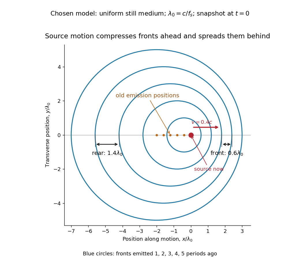
Moving-source wavefront spacing in the classical Doppler effect for sound
. Original linear acoustics model at , with a deliberately enlarged speed ratio for readability. Lengths are measured in . Successive circles are sections of spherical wavefronts emitted one wave period apart; their centres stay at the old emission positions. The forward spacing is and the rear spacing . These chosen parameters differ from the worked example. Details.A receiver approaching a stationary source at instead has , , giving . Moving away gives . The equal closing speeds do not make these equal to the moving-source values. If both source and receiver move together with , however, the numerator and denominator cancel and . For speeds small compared with , the first-order shift is ; the difference between moving-source and moving-receiver experiments appears beyond this first order.
In the same uniform stationary sound model, let be emission time, reception time, and and source and receiver positions. The direct-path propagation condition and its direction areThe unit vector points from the source's old emission position to the receiver's reception position. With velocities and , taking a derivative of the propagation condition givesHere the dot products project onto the actual propagation direction. The last equality counts source wave phase cycles at reception for constant emitted frequency . It assumes both speeds are below , a unique direct arrival and smooth motion; interpreting a measured short-window frequency spectrum additionally requires little frequency change within that window. The source velocity must be evaluated at emission, not at reception. This delayed geometry matters when the direction changes.
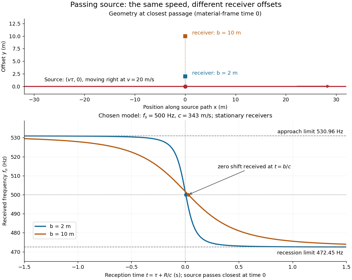
For an original pass-by model, a source follows and a stationary receiver is at with . The source passes its closest position at emission time . ThenThese parametric equations give received frequency against reception time. For the shift is positive, for negative, and the unshifted emission at reaches the receiver at . Thus zero shift occurs after the source's geometric closest passage in the material's reference frame. Increasing spreads the transition over a longer interval even though is unchanged. Far before and after passage, the frequency approaches and respectively.
UNSW School of Physics documents a Doppler effect experiment using a buzzer based on piezoelectricity, powered by a taped-on battery, and a computer's built-in microphone. Audacity records the acoustic wave. First record the stationary source to establish its baseline frequency; then attach it to a bicycle passing the stationary microphone. The published spectrogram shows a rapid decrease in frequency during passage.[ref]
Measuring velocities using the Doppler Shift at UNSW School of Physics. UNSW, Measuring velocities using the Doppler Shift: Introduction, Figs. 1–2; Circular Motion, Measurements (2)–(3); Linear Motion:Bicycle, Moving Source
For numerical readout, select an approaching or receding interval, display its frequency spectrum using Plot Spectrum, and read the interpolated Peak frequency. The protocol recommends repeating with slightly different selections to test stability, and working outdoors to reduce reflections and standing waves. Longer windows refine frequency spacing while averaging over more motion. The baseline controls for the source's actual tone; repeated selections expose analysis-window sensitivity.[ref]
Measuring velocities using the Doppler Shift at UNSW School of Physics. UNSW, Introduction, final paragraph; Circular Motion, spectrogram resolution discussion; Linear Motion:Bicycle, Plot Spectrum and Peak instructions
Under nearly collinear constant-speed approach, infer from the classical Doppler effect for sound. For recession the positive speed is . These inversions need a specified speed of sound. An offset path changes the projection, as in Doppler frequency along a trajectory; neither inversion measures the full speed near closest passage. The protocol's controls cannot remove arbitrary acceleration, background measurement noise or unresolved reflected paths. No new measurements are claimed here.
Articles by others on the same topic



The Doppler effect is a phenomenon observed when the source of a wave (such as sound or light) is moving relative to an observer. It describes the change in frequency (or wavelength) of the wave as perceived by the observer due to the relative motion. 1. **Sound Waves**: When a sound source moves towards an observer, the sound waves get compressed, resulting in a higher frequency (or pitch) of the sound.