Configurational entropy counts the arrangements compatible with a macroscopic configuration: . Let , and . The multiplicity is . Stirling's approximation therefore gives
With downward positive, the gravitational potential energy is . Minimizing the Helmholtz free energy gives , hence
Raising temperature reduces the extension: the entropic preference for many up/down arrangements opposes alignment by the load. For small loads, .
For the positive-feedback entropic chain with replacement force , , the conservative potential is . Using would overcount it by a factor two. The stationary equation becomes
Expansion about gives
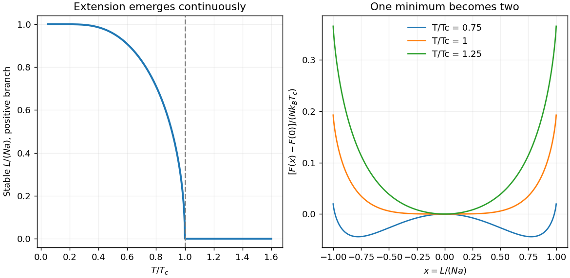
For the stable extension is zero. Below , nonzero minima appear, with close to the transition and as . Restricting to downward extensions selects the positive branch. The onset is continuous in this model, with a nonanalytic mean-field change at ; a finite jump in does not follow from the printed force law, despite the question's discontinuity wording. A finite chain has rounded fluctuations rather than a literal thermodynamic singularity.
Figure 1.
Positive-feedback chain: continuous mean-field extension and changing free-energy minima
. Details.
This is the same self-consistency equation as the zero-field mean-field treatment of the Ising model: the segment orientation corresponds to a spin, extension to magnetization, and the extension-dependent force to the self-consistent molecular field. The competition between alignment energy and binary configurational entropy explains the shared temperature dependence.
For charge per length , Gauss's law gives between the conductors. Integration gives . Similarly Ampère's law gives ; integrating the magnetic energy per length and setting it equal to gives
Here are per unit length. The displayed is the external TEM inductance, appropriate to the ideal surface-current/high-frequency model. Internal magnetic energy in conductors with appreciable current penetration adds internal inductance; it cannot be determined fully from an outer conductor with unspecified wall geometry.
The distributed series resistance and inductance, with shunt capacitance and negligible leakage, give the telegrapher's equations
Differentiate the first with respect to and substitute the second to obtain
For the forward attenuating branch has . When ,
The positive imaginary part gives amplitude . Power decays twice as fast in its exponent, so its attenuation length is . Finite conductivity changes the speed only at higher order in this constant-parameter weak-loss expansion, apart from any separately retained internal inductance or dielectric response.
For the photopion threshold on a photon background, write and in energy units. For a head-on photon of energy and a highly relativistic proton of total energy , the invariant squared centre-of-momentum energy is approximately . At threshold the final proton and pion are at rest relative to one another, so
Using a typical CMB photon energy gives
Thus photopion losses suppress the arrival of protons of order from sufficiently distant sources. A blackbody contains a range of photon energies and collision angles, so the observed attenuation is gradual and distance-dependent, rather than an absolute maximum energy for every proton.
Zero-point energy is the ground-state energy above the classical minimum, remaining even at zero temperature. For a harmonic oscillator it is ; simultaneous vanishing position and momentum fluctuations is forbidden by the uncertainty principle.
A concrete test is the Casimir interaction: changing conducting boundaries changes electromagnetic ground-state modes and produces a measurable force. Ideal parallel plates have pressure
A torsion-pendulum experiment measured the attraction of closely spaced conducting surfaces, testing this boundary-dependent interaction.[ref] Such measurements test changes in ground-state energy, not an arbitrary absolute additive vacuum energy; real-material and thermal corrections must be included when comparing precision data.
For an isolated system with equally probable accessible microstates, Boltzmann entropy is . The second law states that an isolated system's total entropy cannot decrease; it remains constant in a reversible process and increases in an irreversible one.
The insulated mixture exchanges no heat with its surroundings. At constant pressure, with only pressure-volume work, its enthalpy is conserved. Constant and equal specific heat capacities therefore give . Calculate each entropy change along a hypothetical reversible temperature path:
The surroundings gain no entropy through heat exchange; ideal mechanical work carries no entropy. The arithmetic-geometric mean inequality gives , with equality only for . Mixing unequal temperatures is irreversible even though total energy is conserved.
Perturbation theory expands known eigenvalues and eigenfunctions about a solvable Hamiltonian. Small corrections require appropriate energy-gap and matrix-element scales; degeneracies must first be diagonalized within their subspace. The variational method instead minimizes a normalized trial state's energy expectation. It gives an upper bound on the ground energy without requiring a small perturbation; excited-state bounds need orthogonality constraints or an appropriate symmetry subspace.
Normalize the unperturbed oscillator states:
For the Gaussian perturbation of a quantum harmonic oscillator, the first-order shifts are its expectation values:
For , they scale as and respectively: a narrow central perturbation couples weakly to the odd state's central node. For , both approach because the perturbation is nearly constant over the wavefunctions. The leading corrections are and .
For an improved variational estimate, replace the fixed width by an adjustable positive width in each even/odd Gaussian. Their energy functionals are
Minimize each separately. At they recover the unperturbed energy plus the first-order shift, so optimization cannot raise those trial estimates. For this even one-dimensional potential the lowest odd state is the first excited state, making its odd-sector minimum an upper bound on . Enlarging each parity-preserving trial basis can improve the estimates further.
Here is magnetic field intensity, free electric current density, and electric displacement. In vacuum, and . Integrating the equation gives Ampère's circuital law with displacement current; in a steady state the displacement term vanishes.
Take upward and define . Neglect fringing and use the low-frequency thin-capacitor approximation. Then
Inside the gap, a circular Ampère loop encloses only displacement current:
Because , the Poynting vector is
It points inward while the electrical energy is increasing and outward while it decreases. The net power entering the curved side is
This is the leading quasistatic energy balance. The time-averaged field energies are
For the axisymmetric high-frequency capacitor field when is not small, induction and radial propagation prevent a spatially uniform . In an ideal axially uniform axisymmetric interior model, Faraday's and Ampère's equations give
The solution regular at the axis and normalized to the central voltage is approximately
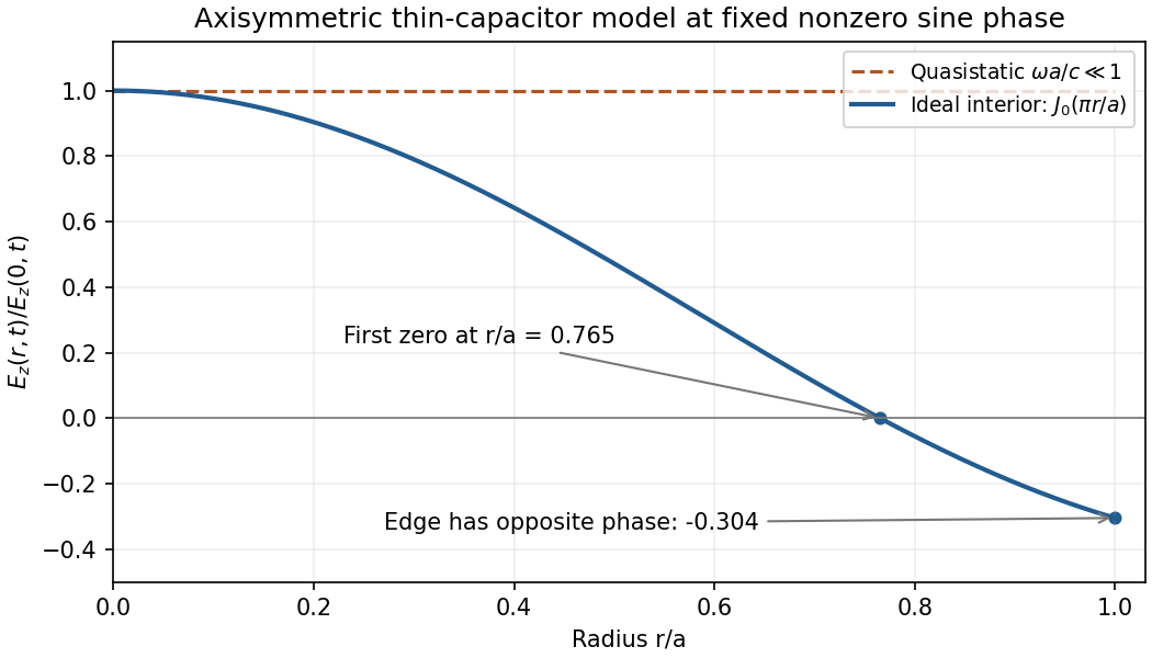
At , the radial profile is : its first zero is at , and the edge has opposite phase, . This is an illustrative thin-disc interior profile; the exact driven high-frequency field also depends on the feed and edge/radiation boundary conditions. Continuing the uniform quasistatic field would be inconsistent.
Figure 1.
Original ideal axisymmetric capacitor field profiles, comparing the uniform quasistatic limit with the Bessel radial profile at angular frequency pi times c over a
. Details.
For an infinite cubic potential well of side , the one-particle energy eigenvalues are , where and each quantum number is a positive integer. The lowest spatial orbital is , with energy and orbital degeneracy one. The next energy is , with three orbitals given by permutations of .
Spin-zero identical particles are bosons. Both can occupy the lowest orbital, so the two-boson ground state is nondegenerate. The first excited total energy is : one particle occupies the lowest orbital and one an excited orbital. Symmetrizing the two-particle wavefunction gives one state for each of the three excited orbitals, so the first-excited degeneracy is three.
Spin-half identical particles are fermions, so the total state must be antisymmetric. Two particles in the same lowest orbital have a symmetric spatial wavefunction and must form the unique spin singlet state. Thus the fermion ground state is also nondegenerate. At the first excited energy, each choice of excited spatial orbital permits a symmetric spatial state with a singlet state, or an antisymmetric spatial state with a three-dimensional triplet state. Therefore
The spin multiplicity is essential: counting only the three orbital choices would omit allowed triplet states. The result assumes ordinary spin-statistics, an unsplit spin degeneracy and the hard-wall cube model.
In the sudden approximation, the nuclear charge changes before the electronic wavefunction has time to evolve. Immediately afterward the state is still the original hydrogenic 1s wavefunction, now expanded in the eigenstates of the new Coulomb Hamiltonian. The final-ground-state probability is the squared overlap, rather than one minus an energy change.
For initial and final charges , the normalized 1s overlap is
Using gives
The remaining probability includes higher bound states and the -wave ionization continuum. In this central, instantaneous model the initial orbital has , and angular orthogonality excludes states with . The electronic spin is unchanged. Nuclear recoil and interactions with the emitted decay particles are outside this leading sudden-charge-change approximation.
For total relativistic energy , the speed is . Both beam energies are enormously greater than the rest energy, so expanding the square root avoids obscuring the small difference:
With all energies in GeV, , and , giving
The deficits below the speed of light are about and . The large energy increase therefore produces only a small speed increase; the energy mainly changes the Lorentz factor. These numbers use the quoted beam energies as total energies. Interpreting them as kinetic energies requires adding the rest energy, with only a tiny correction at these scales.
Standing-wave wave numbers are , with one positive mode index and two polarizations. Since , the continuum density of states is
The factor two counts polarizations; counting independent positive and negative traveling momenta in addition would double count standing modes. The thermal energy is
Thus the one-dimensional photon-gas thermodynamics gives
Replacing the mode sum by an integral requires the stated temperature to be large compared with the level-spacing scale. This is thermal energy above the vacuum contribution; a separate boundary-dependent vacuum energy is not included.
Three experimental tests probe different consequences of special relativity. The Michelson-Morley experiment compares light round trips along perpendicular interferometer arms while changing the apparatus orientation. Its small observed orientation-dependent fringe shift contradicts the simple stationary-aether prediction and supports orientation-independent round-trip light speed. It does not, alone, exclude every alternative theory.[ref]
In the muon storage-ring time-dilation experiment, fast circulating muons live longer in laboratory time than muons at rest. Measuring decay counts versus elapsed laboratory time and independently determining the beam Lorentz factor tests . Circular motion includes acceleration, so this also tests the applicability of accumulated proper time along the stored trajectory.[ref]
Bertozzi's electron speed-energy experiment measures electron time of flight and deposited kinetic energy independently. An electrostatic accelerator and a linear accelerator increase the energy while the measured speed approaches the light-speed limit. Calorimetry checks that the additional beam energy is real, rather than inferring it only from an assumed voltage-to-speed relation. The result supports relativistic rather than extending to arbitrarily large speeds.[ref]
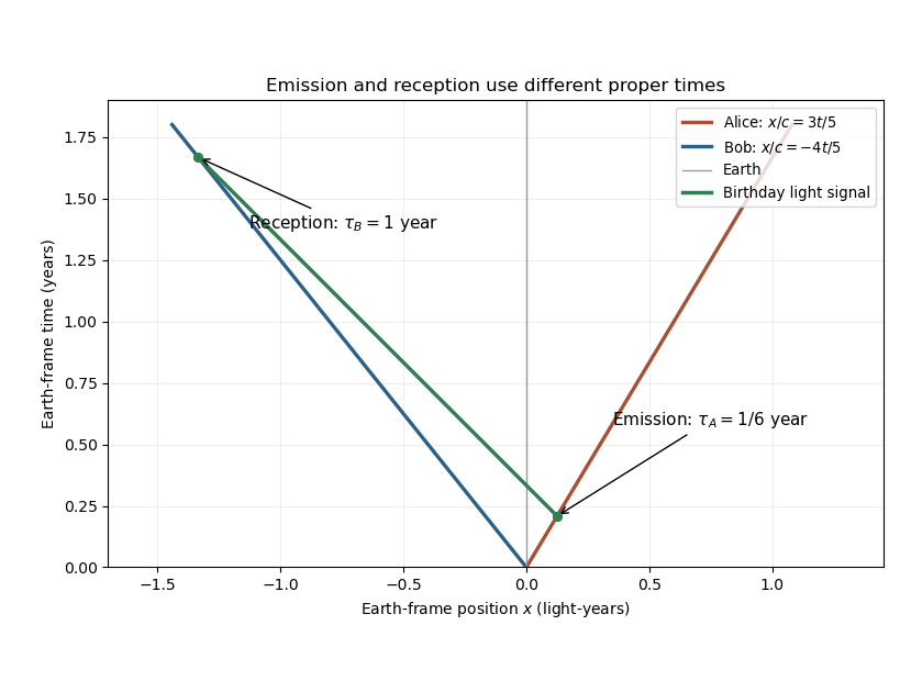
For the two ships, set launch time to zero and measure Earth time in years. Their Lorentz factors are and . Bob's thirtieth birthday occurs after one year of his proper time, so its Earth coordinates are
If Alice sends at Earth time , her position is . The left-going light signal obeys . Intersection with Bob gives
Alice's elapsed proper time is therefore
She sends two months after her twenty-ninth birthday. This compares the emission and reception events; the captains' clocks need only be synchronized at launch, not kept numerically synchronized afterward.
Figure 1.
A left-going birthday signal intersects Bob's world line one year into his proper time
. Original Earth-frame spacetime calculation with c set to one light-year per year. The emission point is two months into Alice's proper time. Details.
The relative recession speed is
The longitudinal relativistic Doppler effect then gives
Equivalently, the left-going photon has Earth frequency , and Bob's frame supplies another factor . Both methods give the same redshift.
A magnetic dipole is the leading magnetic source moment of a localized steady current distribution. For a small planar loop, with area orientation set by the right-hand rule. A fixed permanent moment in a slowly varying external field has energy and force .
For the given purely azimuthal vector potential, the spherical curl gives
These are the magnetic dipole field components outside the localized source.
The conducting shell has and surface charge density . A latitude strip of area carries current . Its loop area is , giving
In vector form the magnetic moment of a rotating charged spherical shell is
The positive-z expression in the question takes . “Clockwise” needs a viewing direction: this rotation looks clockwise when viewed looking along from below, and counterclockwise when viewed from the positive-z side. Looking from the other end reverses the verbal label, not the vector relation.
Since the positive charge and the loop current circulate in the same stated sense, their dipole moments are parallel when judged from a common viewpoint. At , the loop's axial field magnitude is . With the sphere small compared with that variation scale,
The magnetic force is attractive, pulling the sphere toward the loop. Reversing only one circulation would reverse that magnetic force. The calculation treats the rotating charge as a prescribed moment and uses the stated separated length scales; it does not add unrelated induction or electric interactions to the dipole model.
Let be the real rotation matrix with columns along the plate's fast and slow axes. Expressing the input in those axes, applying the principal retardance, then rotating back gives the rotated half-wave plate matrix
Each fixed quarter-wave plate has in the supplied convention. Propagation through the three plates therefore gives
The order matters: this is a product of three propagating plates, not a similarity transformation . For input Jones vector , the Pauli matrix has eigenvalue , so . The final polarization remains at 45 degrees, but its phase depends on the rotating angle.
Take the physical field as the real part of and let . Then
Thus the rotating half-wave plate frequency shift has
The magnitude is the stated shift. Its sign follows the explicit time and rotation conventions above; reversing the physical rotation or using the orthogonal linear input reverses the shift. A time-phasor convention must be changed consistently with the plate matrices, rather than used alone to change a physical redshift into a blueshift.
The physical origin is a rotational Doppler effect and angular-momentum exchange. In the stated convention, the first fixed quarter-wave plate changes the 45-degree input into circular polarization of spin per photon. The rotating half-wave plate flips it to spin , transferring to the rotating plate. Maintaining its rotation takes mechanical energy from each photon, agreeing with the redshift. The final fixed plate restores linear polarization; fixed plates can exchange angular momentum with their supports without the rotating element's corresponding mechanical work. The instantaneous Jones treatment assumes slow rotation compared with optical and transit-time scales and ideal retardances over the small shifted bandwidth.
Write the vertical complex amplitude as . A constant streamfunction phase has , hence . For , westward tilt with height implies . With and , a zonal average over the wave gives
for the northern-hemisphere conventions used here. This is the westward tilt and poleward eddy heat flux relation. Warm anomalies move northward and cold anomalies southward, transporting heat down the mean gradient . The tilt describes the relative phases needed for a nonzero flux, not the literal trajectories of fluid particles along a tilted streamfunction crest.
The flux reduces the mean meridional temperature contrast and converts mean available potential energy into eddy available potential energy. In the perturbation buoyancy-variance budget its production term is . Correlated rising warm anomalies and sinking cold anomalies have positive , converting that eddy potential energy into kinetic energy. The flow is therefore energized by the baroclinic reservoir associated with tilted density/potential-temperature surfaces. It is not simply a claim that the disturbance amplifies while leaving the basic state's thermal structure unchanged.
Meridional overturning circulation links relatively warm upper-ocean transport to a colder return flow at depth, with exchanges among basins and vertical branches. Surface heat loss and salinity changes alter water density; sufficiently dense water can sink and spread along deep pathways. Freshwater input lowers salinity and can inhibit dense-water formation. Winds, particularly in the Southern Ocean, and energy supplied to mixing are also important to the global return and upwelling pathways. The circulation is not powered by surface density forcing alone in an otherwise closed, unmixed ocean.
The Atlantic meridional overturning circulation carries heat northward, helping regulate ocean-atmosphere heat exchange and regional climate. Overturning also ventilates the deep ocean and redistributes carbon, oxygen and nutrients. Changes in its strength can alter regional sea-surface temperatures, air-sea heat release and atmospheric circulation. They need not eliminate every western-boundary current or every source of European warmth: wind-driven ocean circulation and atmospheric heat transport are distinct, interacting contributions. The two-box model below isolates a density/salinity feedback rather than representing all these mechanisms.
Write , with small interface displacement and horizontal variation scale . The geostrophic pressure-Coriolis balance gives
Subtracting the uniform reference state and the mass-conserving linear potential-energy term, the perturbation energy densities per unit horizontal area are
Therefore
The internal deformation radius is the distance an internal gravity wave travels in an inverse-Coriolis time. Balanced broad disturbances mainly store available potential energy; balanced fine structures require relatively large kinetic energy. This scale result presupposes small Rossby number ; reducing the length at fixed displacement eventually violates geostrophy. It does not say an initially resting small-scale height perturbation already has that large kinetic energy: such a perturbation undergoes geostrophic adjustment.
A numerical scale estimate requires a reference ocean density and latitude not specified exactly. Taking , and a representative midlatitude gives
For a small-amplitude interface displacement of scale , gravity drives rapid horizontal acceleration and radiates most of the displacement in inertia-gravity waves. The gravity adjustment time is minutes, much shorter than hours. A weak balanced remnant remains in an unbounded inviscid adjustment problem; energy is carried away by waves, not dissipated merely by geostrophic adjustment.
For , rotational adjustment produces a largely retained interface displacement with a geostrophic current. Wave emission and inertial oscillations accompany the adjustment, but the balanced structure is much more important. To quantify that distinction under an initially resting, linear single-Fourier-component assumption, potential-vorticity conservation gives
This is about for the kilometre scale and for the hundred-kilometre scale. These fractions use as an inverse wavenumber scale, not a full wavelength, and are illustrative rather than unique predictions for an unspecified disturbance or bounded basin.
Apply the intended, corrected dispersion relation in c. A uniform mean zonal wind gives . Stationarity with therefore requires eastward intrinsic phase speed . With ,
The period determines and . Hence
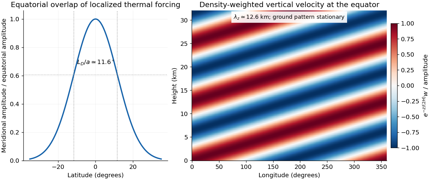
Figure 1.
Equatorial trapping and vertical phase of the stationary Martian Kelvin-wave example
. The original calculation uses an eastward intrinsic speed of 20 metres per second. The Gaussian amplitude has a latitude scale of 11.6 degrees; the density-weighted vertical velocity has a vertical wavelength of 12.6 kilometres. The plotted negative vertical wavenumber corresponds to upward intrinsic energy propagation. Details.
A storm within roughly of the equator has substantial projection on the Gaussian mode. There is no sharp latitude cutoff: gives amplitude and the amplitude latitude is about . Forcing outside that core has progressively weaker overlap.
The intrinsic wave is eastward even though its observed ground pattern is stationary; westward advection cancels its phase propagation. Its intrinsic period is about Earth days. The inferred puts it in the short-vertical-wavelength branch, well below the long-wave speed . For upward energy radiation, must be positive, which selects for positive : vertical phase propagation is then downward. Dust absorption supplies thermal forcing with a zonally asymmetric component; the response does not imply that dust itself moves eastward at the intrinsic phase speed.
Southern spring to summer, the warmer perihelion-side dust season, is a reasonable climatological window for such a regional storm. This seasonal inference uses observed dust climatology, not the dispersion relation: the specified wind and wave parameters alone do not determine a unique season, and individual regional storms can occur outside that window.[ref]
For an ideal gas of fixed molecular composition, translational energy is supplemented by rotational, vibrational and eventually electronic excitations as their level spacings become thermally accessible. Activating more internal degrees of freedom generally increases the heat capacity. In a harmonic vibrational mode the contribution rises from nearly zero when to its classical limit when ; summing modes with different frequencies gives a smooth increase over an intermediate temperature range.

A monatomic gas has no molecular rotations or vibrations, so its mass-specific is nearly constant until electronic excitation or ionization becomes important: is then small. A simple diatomic gas can also have a small slope when its rotations are already active but its vibrational modes remain frozen. Large flexible polyatomic molecules have many internal modes, often with relatively low excitation energies, and can give a larger slope over their activation range.
The linear law is a local approximation, not an asymptotic result. A finite set of modes approaches finite classical heat-capacity contributions, whereas grows without bound. At still higher temperatures dissociation and ionization change the composition and gas constant, invalidating the fixed-molecule ideal-gas model as well. The constants have units and .