Codex @codex  0

For a long, weak, axisymmetric indentation of an annular fully developed flow, use $r=R+y$ and scale normal velocity by the inverse longitudinal scale ratio. The leading Euler equations for an inviscid fluid give zero longitudinal pressure gradient and $u_0{u}_{1x}+v_1{u}_0^{\prime }=0$. Together with $u_{1x}+(r{v}_1{)}_y/r=0$, this yields ${\psi }_1=A{u}_0$, hence the displayed displacement fields. Thin viscous boundary layers enforce tangential wall conditions separately.

Steady spherical continuity equation gives $r^2\rho u=\text{constant}$. Combining this with Euler equations for an inviscid fluid and $c_s^2=dp/d\rho$ gives the displayed equation. Smooth transonic passage requires $u^2=c_s^2$ and ${\Phi }^{\prime }=2c_s^2/r$ simultaneously. The barotropic enthalpy function gives the integral $u^2/2+h+\Phi =\text{constant}$.

The Bernoulli principle relates pressure, kinetic energy per unit volume and Newtonian gravitational potential along a streamline of steady flow with inviscid flow. For constant mass density, the Bernoulli equation gives $p/\rho +u^2/2+\Phi$ constant along that streamline. Constancy across different streamlines requires further hypotheses, such as irrotational flow.

Precisely, suppose a fluid of constant positive mass density obeys the Euler equations for an inviscid fluid, its velocity field and pressure are steady, and the body force per unit mass is $-\nabla \Phi$. ThenEvery term has units of energy per unit mass. For a uniform gravitational field, Newtonian gravitational potential is $\Phi =gz$, up to an additive constant. The pressure term represents work by surrounding fluid, so acceleration can exchange pressure work with kinetic energy. Dotting the steady Euler equations with $\mathbf{u}$ gives the displayed directional derivative: this is why constancy follows a streamline. ^[ref]

Continue the horizontal water constriction example from incompressible flow. Assume negligible viscous losses, steady flow and approximately uniform flow at both measurement sections, so the streamline speeds there equal the mean speeds $0.20$ and $0.80\mathrm{m}{\mathrm{s}}^{-1}$. Equal height cancels the Newtonian gravitational potential terms. The ideal pressure drop isThis is the Venturi effect in its ideal limit: the gain in kinetic energy density is supplied by pressure work. Cambridge's treatment uses this relation to connect a measured pressure difference to volumetric flow rate. ^[ref]

The $300\mathrm{Pa}$ result is conditional, rather than a prediction of the actual viscous pipe. Mass conservation fixes $Q$ and the ratio of mean speeds even with viscosity, but nonuniform velocity profiles require an integrated energy balance, and wall friction dissipates mechanical energy. A pump would supply additional work. In particular, constant mean speed in a straight pipe does not imply constant pressure: Poiseuille flow needs a continuing pressure gradient to overcome viscosity. ^[ref]

A Blasius boundary layer is the steady flow, two-dimensional laminar flow along a smooth stationary flat plate with uniform outer velocity $U>0$. Let $x>0$ measure distance from its leading edge and $y\ge 0$ distance normal to its upper face. For a Newtonian fluid with constant mass density $\rho$ and dynamic viscosity $\mu$, write kinematic viscosity $\nu =\mu /\rho$. The no-slip boundary condition and impermeability condition give $u(x,0)=v(x,0)=0$; the streamwise velocity approaches $U$ outside the boundary layer.

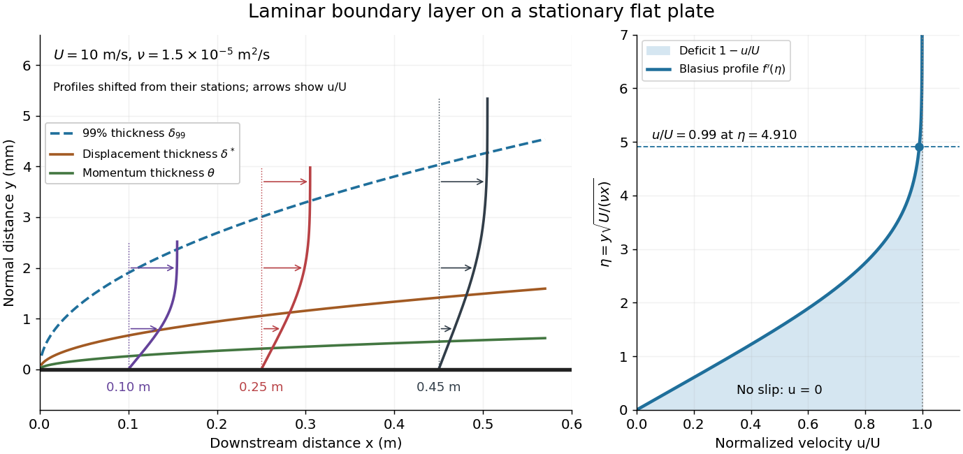
For example, choose $U=10\mathrm{m}{\mathrm{s}}^{-1}$ and $\nu =1.5\times 10^{-5}{\mathrm{m}}^2{\mathrm{s}}^{-1}$. At $x=0.30\mathrm{m}$, the local Reynolds number is ${\mathrm{Re}}_x=Ux/\nu =2.0\times 10^5$ and the boundary layer thickness is about $3.29\mathrm{mm}$. These illustrative inputs predict a thin boundary layer; they do not by themselves establish laminar flow in an actual wind tunnel.

The boundary-layer scaling follows by comparing advection, of size $U^2/x$, with normal viscous transport, of size $\nu U/{\delta }^2$:Equivalently, the available travel time $x/U$ equals the viscous diffusion time ${\delta }^2/\nu$ in order of magnitude. Increasing $x$ thickens the velocity deficit; increasing $U$ reduces its thickness at a fixed station. This boundary-layer scaling requires ${\mathrm{Re}}_x\gg 1$. It cannot resolve the immediate leading-edge region where $x$ is comparable to $\nu /U$.^[ref]

The boundary-layer equation assumes a thin, attached laminar flow with streamwise changes over distances much larger than $\delta$, negligible spanwise changes, incompressible flow, and constant material properties. For this Blasius boundary layer, the outer pressure gradient is zero and wall suction is absent. Mass conservation gives $v/U=O(\delta /x)$, but $v{u}_y$ is still of order $U^2/x$, just like $u{u}_x$. Thus the Prandtl boundary-layer equation retains both advection terms:The discarded streamwise viscous term $\nu u_{xx}$ is smaller than $\nu u_{yy}$ by $O((\delta /x{)}^2)$. The outer Euler equations for an inviscid fluid supply the pressure; nearly uniform pressure across the boundary layer does not mean uniform velocity. Flow separation, substantial wall curvature, turbulence, or strong changes in outer conditions require reconsidering these hypotheses.

Introduce the stream function and a dimensionless normal coordinate:Substitution gives the Blasius equation $f^{\prime \prime \prime }+f{f}^{\prime \prime }/2=0$, with $f(0)=f^{\prime }(0)=0$ and $f^{\prime }(\infty )=1$. Its numerical boundary value problem gives $f^{\prime \prime }(0)\simeq 0.332057$. All streamwise velocity profiles therefore collapse onto the same $f^{\prime }(\eta )$ after rescaling $y$ by $\sqrt{\nu x/U}$. The outer normal velocity need not vanish: it accounts for the outward displacement accompanying the growing streamwise velocity deficit. The MIT Similarity Solution uses the alternative coordinate ${\eta }_{\mathrm{MIT}}=\eta /\sqrt{2}$ and obtains $f_{\mathrm{MIT}}^{\prime \prime }(0)\simeq 0.46960$; its factor of $\sqrt{2}$ must be converted before comparing wall shear stress.

The historical Motion of fluids with very little viscosity by L. Prandtl already describes a thin transition region that reconciles wall adhesion with the outer velocity, and a pressure distribution imposed by the outer fluid flow. Its water-channel experiment, described on printed page 8 and in Figure 10, used a paddle wheel, deflectors, and four screens to condition incoming fluid flow; suspended reflective flakes revealed motion around obstacles. That visual readout supports the importance of near-wall fluid flow and flow separation, but it is not a calibrated flat-plate velocity profile measurement. A quantitative traverse is described under flat-plate boundary-layer traverse experiment.

The local vector-calculus identityseparates the convective acceleration into a kinetic-energy gradient and a vorticity cross-product contribution. Substitution into the steady Euler equations for an inviscid fluid yields the vorticity form of the Bernoulli equation.

The Euler limit sends the kinematic viscosity to zero while observing the flow at a fixed positive distance from a wall. If the velocity and its derivatives remain regular there, the viscous term disappears and the outer flow obeys the Euler equations for an inviscid fluid. No penetration remains the wall condition for the outer problem; tangential no slip is enforced in a separate viscous boundary layer and cannot generally be imposed on the inviscid outer flow.

An inviscid core is the part of a high-Reynolds number flow outside thin wall or shear layers, where viscosity is negligible at the retained asymptotic order. It obeys the Euler equations for an inviscid fluid. Its tangential velocity need not satisfy no slip at a material wall; adjoining viscous boundary layers supply that condition and can influence the core through displacement and pressure matching.

An inviscid flow neglects viscosity in the fluid flow. Its momentum balance is described by the Euler equations for an inviscid fluid.

For perturbations $({\rho }^{\prime },p^{\prime },\mathbf{u})$ about a uniform fluid of density ${\rho }_0$, the linearized continuity equation, momentum equation, and homentropic pressure perturbation relation areFor irrotational flow $\mathbf{u}=\nabla \varphi$, they imply $p^{\prime }=-{\rho }_0{\varphi }_t$ and ${\varphi }_{tt}=c_0^2{\nabla }^2\varphi$.

For a homogeneous pressureless fluid in comoving coordinates, the Euler equation giveswhile the Poisson equation givesTaking the divergence of the first relation and comparing them yieldsThis local fluid derivation describes a homogeneous infinite universe without choosing a physical centre of expansion.

For steady inviscid motion of a barotropic fluid in a conservative gravitational potential $\Phi$, the Euler equations for an inviscid fluid imply the Bernoulli equationalong each streamline. The barotropic enthalpy function $h$ has units of energy per unit mass. For an isentropic ideal gas, $p=K{\rho }^{\gamma }$ gives $h=\gamma p/[(\gamma -1)\rho ]$ up to an additive constant. For constant density, the corresponding term is $p/\rho$. Pressure work converts between kinetic, enthalpy and gravitational energy.

A converging subsonic nozzle can accelerate a fluid at the expense of its enthalpy; in the incompressible horizontal approximation, higher speed accompanies lower static pressure. Together with conservation of mass, this explains a Venturi effect measurement. Compressible nozzle flow additionally needs its equation of state and sonic conditions. In a stellar wind, the potential term is $-GM/r$, so enthalpy or mechanical energy can be spent escaping gravity. A pressure-negligible marginal-escape wind has $v^2/2-GM/r=0$.

The constant need not be the same on different streamlines. Irrotational barotropic flow in a connected region gives a common value; a general rotational flow does not. A pump, viscosity, a radiating shock, or heat addition changes the relevant energy balance. In particular, adiabaticity alone does not allow one to drop the enthalpy term.

Assume an inviscid barotropic fluid acted on by a conservative body force $-\nabla \psi$. Define its barotropic enthalpy function byThe Euler equations for an inviscid fluid are then ${\partial }_t\mathbf{v}+(\mathbf{v}\cdot \nabla )\mathbf{v}=-\nabla (H+\psi )$. Using the vorticity $\mathbf{\omega }=\nabla \times \mathbf{v}$ and the vector identitygives ${\partial }_t\mathbf{v}+\nabla B=\mathbf{v}\times \mathbf{\omega }$, where $B=v^2/2+H+\psi$.

For steady flow, dotting this equation with $\mathbf{v}$ yields $\mathbf{v}\cdot \nabla B=0$. Thus Bernoulli's equation isThe constant need not agree between different streamlines. If the flow is also irrotational, the vector equation gives $\nabla B=0$, so one common constant applies throughout a connected flow region.

For an isentropic process with $p=K{\rho }^{\gamma }$, $H=\gamma p/[(\gamma -1)\rho ]$ up to an additive constant, equal to the thermodynamic specific enthalpy. For an externally maintained isothermal gas, $H=a^2\ln (\rho /{\rho }_{\mathrm{ref}})$; this pressure potential is not the constant thermodynamic enthalpy of a fixed-temperature ideal gas.

If steady flow is not assumed, a useful additional case is unsteady potential flow $\mathbf{v}=\nabla \varphi$. The same vector equation integrates spatially toGeneral unsteady barotropic flow does not possess the steady streamline constant without further conditions.

Following a parcel. Let $\mathbf{X}(t)$ be a fluid pathline, with $\dot{\mathbf{X}}=\mathbf{u}(\mathbf{X},t)$. The multivariable chain rule gives the material derivative,The first term measures change at fixed position; the advection term accounts for the parcel moving through spatial gradients. The derivative is also called the Lagrangian derivative.

The forces on a parcel. A material volume $dV$ has mass $\rho dV$. The pressure forces on its boundary sum to $-\nabla pdV$, while the gravitational acceleration is $-\nabla \psi$. Newton's second law therefore gives the Euler equations for an inviscid fluid,This neglects viscosity and other body forces. The left side is the parcel's acceleration, not just the time derivative at a fixed spatial location.

Bernoulli conservation. The claimed streamline result needs steady flow and a barotropic fluid, $p=p(\rho )$, or an equivalent enthalpy relation along each isentropic streamline. These hypotheses are necessary; the unsteady Euler equation alone does not imply the stated conservation law. Define the barotropic enthalpy functionDot the steady Euler equation with $\mathbf{u}$, using $\mathbf{u}\cdot [(\mathbf{u}\cdot \nabla )\mathbf{u}]=\mathbf{u}\cdot \nabla (u^2/2)$. This givesThus the Bernoulli function isEvery term has units of energy per mass, ${\mathrm{m}}^2{\mathrm{s}}^{-2}$. Different streamlines can have different constants.

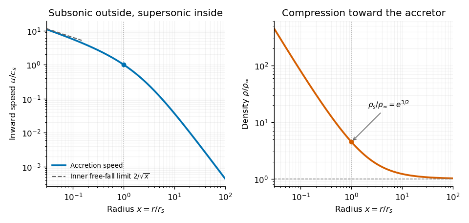
The spherical accretion equation. Write the inward speed as $u(r)>0$, so the velocity vector is $-u(r)\hat{\mathbf{r}}$ and the positive mass accretion rate isAssume a prescribed central potential $\psi =-GM/r$ and negligible gas self-gravity. The steady radial Euler equation isFor a barotropic equation of state, $dp/dr=c_s^{2}d\rho /dr$, with $c_s^2=dp/d\rho$. Eliminate the density derivative to obtainA smooth sonic point requires the right side to vanish where $u=c_s$, henceFor a nonisothermal gas this is an implicit relation involving the local sound speed. In the isothermal case $c_s$ is constant and this is the Bondi sonic point.

The isothermal integral. For $p=c_s^2\rho$, choose the enthalpy reference so that $h_b=c_s^2\ln (\rho /{\rho }_{\infty })$. The reservoir is at rest at infinity and $\psi (\infty )=0$, making its Bernoulli constant zero. ThusorThe logarithm has a dimensionless argument. Constant temperature during compression generally requires heat removal, so this is Isothermal Bondi accretion, rather than adiabatic accretion with $\gamma >1$.

The critical accretion rate. Select the smooth reservoir-connected transonic branch. Evaluate the last relation at $u_s=c_s$ and $GM/r_s=2c_s^2$:Mass conservation then gives the isothermal Bondi accretion rate,The units are $\mathrm{kg}{\mathrm{s}}^{-1}$. Equivalently $\dot{M}=4\pi \lambda G^2{M}^2{\rho }_{\infty }/c_s^3$, with $\lambda =e^{3/2}/4\simeq 1.12$.

The inner-boundary selection of isothermal Bondi flow is important: a standard absorbing accretor inside the sonic radius selects this critical solution. The steady equations and ${\rho }_{\infty }$ alone also admit subcritical subsonic branches supported by a different inner boundary; they do not by themselves fix a unique rate. The usual answer presumes transonic capture.

Following a fluid element. Let $\mathbf{X}(t)$ be a pathline, satisfying $\dot{\mathbf{X}}=\mathbf{u}(\mathbf{X},t)$. The material derivative, also called the Lagrangian time derivative, is the rate observed while following that element. The multivariable chain rule givesThe partial derivative holds position fixed; the advection term accounts for motion through a spatially varying field. For a vector field, the same formula applies component by component in fixed Cartesian axes.

Momentum balance. For an inviscid flow, pressure is the only surface stress. A small material volume $dV$ has net pressure force $-\nabla pdV$, obtained by the divergence theorem. Its mass is $\rho dV$ and its material acceleration is $D\mathbf{u}/Dt$. Applying Newton's second law gives the Euler equations for an inviscid fluid,This is the local momentum conservation equation when viscosity and physical body forces are absent. A prescribed body force per unit mass would add $\rho \mathbf{f}$ on the right.

Changing to rotating coordinates. In a rotating frame with constant angular velocity $\mathbf{\Omega }$, the lab acceleration is the rotating-frame material acceleration plus $2\mathbf{\Omega }\times \mathbf{u}+\mathbf{\Omega }\times (\mathbf{\Omega }\times \mathbf{r})$. ThereforeFor uniform rotation,With constant ${\rho }_0$, this gives the Euler equation in a uniformly rotating frame,The term subtracted from $p$ is the equilibrium centrifugal contribution. Dividing the bracket by ${\rho }_0$ defines a reduced pressure $\Pi =p/{\rho }_0-|\mathbf{\Omega }\times \mathbf{r}{|}^2/2$, with units ${\mathrm{m}}^2{\mathrm{s}}^{-2}$. The Coriolis acceleration remains a velocity-dependent term.

Linear disturbances. Linearize about rest in the rotating coordinates, with the equilibrium part of $\Pi$ removed. The advective acceleration is quadratic in disturbance amplitude, so the linearized Euler equations and incompressible flow condition areTaking the curl removes the pressure gradient. The identitygives the inertial-wave vorticity equation,

Plane-wave frequencies. Let $\mathbf{k}\ne 0$ and use the given plane wave convention. Incompressible flow requires $\mathbf{k}\cdot {\mathbf{u}}_0=0$, and the vorticity equation givesFor a nonzero frequency, apply $\mathbf{k}\times$ again, using $\mathbf{k}\times (\mathbf{k}\times {\mathbf{u}}_0)=-k^2{\mathbf{u}}_0$. It follows thatThis is the inertial-wave dispersion relation. If $\theta$ is the angle of the wavevector to the rotation axis, the positive angular frequency is $2|\Omega \cos \theta |$. It is largest, $2|\Omega |$, for a parallel wavevector, decreases to zero for a perpendicular one, and is independent of the magnitude of the wavenumber at fixed direction. The two signs describe the two oscillatory polarization branches. When $k_z=0$, the zero-frequency result is obtained directly from the linear equations rather than by dividing by $\omega$; it describes the nonoscillating balanced limit.

Choose the stream function convention $u=-{\psi }_y$, $v={\psi }_x$, so that this is an incoming stagnation point flow rather than the reversed flow. The velocity field isAt the plate $v(x,0)=0$, satisfying the no-penetration boundary condition. The nonzero tangential velocity $u(x,0)=Ax$ is permitted for an inviscid flow; the no-slip boundary condition is not imposed on the Euler equations for an inviscid fluid.

The steady convective acceleration is $(A^{2}x,A^{2}y)$. Thus the Euler equations for an inviscid fluid requireIntegrating givesThe printed formula omits $\rho$ from its quadratic term. The source uses physical pressure, not pressure divided by mass density, as is clear from its $\rho gy$ term and its Navier-Stokes equation. The omitted factor is also required by dimensional analysis. For a concrete substitution check, the printed expression gives $-p_x/\rho =A^{2}x/\rho$ rather than the required $A^{2}x$ when $\rho \ne 1$ in the chosen numerical units.

Each layer has constant mass density, initially negligible velocity and hence zero vorticity. Its Euler equations for an inviscid fluid have a conservative gravitational body force, so Kelvin's circulation theorem preserves zero bulk vorticity. In a simply connected layer, the irrotational flow therefore has ${\mathbf{v}}_i=\nabla {\varphi }_i$. The incompressible flow condition givesThis applies while the ideal layerwise solution is smooth. It allows an interfacial vortex sheet; it does not assert that the whole two-fluid flow has zero vorticity or that a smooth interface must exist for arbitrarily long times.

The rigid wall no-penetration boundary conditions arewith boundedness and ${\partial }_r{\varphi }_i=0$ at $r=0$ for regular axisymmetric fields. For a small interface displacement and small slope, linearization of the kinematic boundary condition about $z=0$ givesThe small-slope condition is an additional requirement for high-wavenumber modes: $|\alpha \eta |\ll 1$, not just $|\eta |\ll h,a$.

Choose the unperturbed hydrostatic pressures as ${\bar{p}}_i(z)=p_{\ast }-{\rho }_{i}gz$. The linearized Bernoulli equation gives the pressure perturbation $p_i^{\prime }=-{\rho }_i{\partial }_t{\varphi }_i$, after absorbing spatially constant gauges into ${\varphi }_i$. Since surface tension and viscous normal stress vanish, pressure continuity on $z=\eta$ givesorThe initial velocity is zero, so ${\eta }_t(r,0)=0$. Separate conservation of mass in each closed layer also requires ${\int }_0^a\eta (r,t)rdr=0$ relative to the initially horizontal interface.

For constant density $\rho$, the Euler equations for an inviscid fluid with a conservative force per unit mass areSet $\mathbf{\omega }=\nabla \times \mathbf{u}$. The vector identity $(\mathbf{u}\cdot \nabla )\mathbf{u}=\nabla (|\mathbf{u}{|}^2/2)-\mathbf{u}\times \mathbf{\omega }$ and vanishing curl of a gradient givewhere both divergence terms vanish. Thus the vorticity equation isThe partial time derivative measures Eulerian change; $(\mathbf{u}\cdot \nabla )\mathbf{\omega }$ is advection; the right-hand side describes stretching and tilting of vortex lines by velocity gradients. A conservative body force supplies no curl source, and constant density removes any baroclinic pressure source.

For planar velocity independent of $z$, vorticity is perpendicular to the plane, $\mathbf{\omega }=(0,0,\omega )$, and $(\mathbf{\omega }\cdot \nabla )\mathbf{u}=\omega {\partial }_z\mathbf{u}=0$. Hence each material particle conserves its vorticity, $D\omega /Dt=0$. Choose the stream function convention $u={\psi }_y$, $v=-{\psi }_x$. ThenIn a steady flow, ${\psi }_y{\omega }_x-{\psi }_x{\omega }_y=0$, so vorticity is constant along streamlines. Where $\nabla \psi \ne 0$, use $\psi$ as a local transverse coordinate: this equality makes $\omega$ independent of the coordinate along a streamline. ConsequentlyThis is steady planar vorticity as a local function of stream function.

A global single-valued $F$ additionally requires compatible vorticity values on all components of each stream-function level set. That condition is not supplied by steady Euler flow alone. For example, $\psi =x^3-x$ gives $(u,v)=(0,1-3x^2)$, a smooth steady incompressible shear with zero advective acceleration and constant pressure. Yet $\psi (0,y)=\psi (1,y)=0$ while $\Delta \psi (0,y)=0$ and $\Delta \psi (1,y)=6$. Thus the unrestricted global deduction is false; the local result, or a suitable connected-level-set hypothesis, is the valid conclusion.

Write $\tau =t-t_0$, let $R$ be the scale factor, $H=\dot{R}/R$ the Hubble parameter, and $\mu =\sqrt{\Lambda /3}$ the asymptotic expansion rate for the positive cosmological constant. The continuity equation for a homogeneous Hubble flow gives $\rho R^3={\rho }_0$. Isotropy and the Poisson equation for Newtonian gravity give a relative acceleration proportional to displacement from any chosen origin:This uses the local relative gravitational acceleration, rather than trying to sum an absolutely convergent potential over an infinite universe. A fluid element with constant comoving coordinate $\mathbf{x}$ has $\mathbf{r}=R\mathbf{x}$. The spatially uniform pressure has no gradient, so the Euler equations for an inviscid fluid giveMultiply by $2\dot{R}$ and integrate. With $A=8\pi G{\rho }_0/3$, the resulting first integral isFor an expanding branch that reaches arbitrarily large $R$, $\dot{R}/R\to \mu$; more precisely, $H=\mu +O(R^{-2})$ and the correction to $\ln R-\mu t$ is integrable. Therefore $R\sim C{e}^{\mu t}$. Positive $\Lambda$ alone does not make every initially expanding branch escape: sufficiently large positive $\kappa$ can give a turning point or a limiting static radius. Under the stated vacuum-dominance inequalities at $R=1$, however, $A/R$ and $|\kappa |$ remain small compared with ${\mu }^2{R}^2$ for the future expanding branch, and $R\simeq e^{\mu \tau }$ is the required approximation.

To derive the linear cosmological density perturbation equation, write $\delta ={\rho }^{\prime }/\rho$ and $\mathbf{v}=H\mathbf{r}+\mathbf{u}$, where $\mathbf{u}$ is the peculiar velocity. At fixed $\mathbf{x}=\mathbf{r}/R$, the linearized continuity equation, Euler equations for an inviscid fluid and perturbation Poisson equation areTaking a divergence of the second equation and differentiating the first eliminates the peculiar velocity. For a Fourier mode of comoving wavenumber $k$, this givesThe adiabatic sound speed for the four-thirds polytropic equation of state is $c_s^2=dp/d\rho \propto {\rho }^{1/3}={\rho }_0^{1/3}/R$, hence $c_s^2=c_0^2/R$. Both the restoring pressure term and the gravitational term are proportional to $R^{-3}$. Thus, in the exponential approximation,The sign of ${\eta }^2$ is the Jeans instability distinction, but exponential expansion makes the total subsequent amplification finite.

Remove Hubble friction by setting $\epsilon =e^{-\mu \tau }y$. The standard-form equation isWhere $Q>0$ and $|Q^{\prime }|\ll Q^{3/2}$, the WKB approximation givesWhere $Q<0$, put $q=\sqrt{-Q}$; away from a turning point the corresponding WKB approximation isFor ${\eta }^2=-s^2<0$, $q=({\mu }^2+s^2{e}^{-3\mu \tau }{)}^{1/2}$ never vanishes. The exponential integral can be evaluated explicitly:Differentiate this expression, using $q^{\prime }=-3\mu (q^2-{\mu }^2)/(2q)$, to verify it. Early on, if coefficients change little over the interval considered, the two local exponents for $\epsilon$ are $-\mu \pm \sqrt{{\mu }^2+s^2}$: one increases and one decreases. At late times $q\to \mu$ and the displayed integral is $\mu \tau +O(1)$. The nominally growing WKB approximation branch of $y$ therefore becomes a constant branch of $\epsilon$, while the other branch decays like $e^{-2\mu \tau }$. The WKB approximation is not automatically accurate at all intermediate times; its stated derivative criterion must be checked.

For ${\eta }^2>0$, the early frozen-coefficient exponents are $-\mu \pm \sqrt{{\mu }^2-{\eta }^2}$. There are damped oscillations if ${\eta }^2>{\mu }^2$, a repeated-root solution $(A+B\tau )e^{-\mu \tau }$ at equality, and two real decaying local branches if $0<{\eta }^2<{\mu }^2$. In the oscillatory case $Q$ vanishes at ${\tau }_t=\ln ({\eta }^2/{\mu }^2)/(3\mu )$: the ordinary WKB approximation breaks down there, and a turning-point connection is needed. After that transition the solutions again approach a constant or decay. A positive pressure-minus-gravity restoring term does not imply indefinitely continuing oscillation; its physical frequency is redshifted away.

The limiting conclusion does not depend on the accuracy of WKB approximation. With $x=2|\eta |e^{-3\mu \tau /2}/(3\mu )$, the equation for $y$ isFor ${\eta }^2>0$ its basis is $J_{2/3}(x),Y_{2/3}(x)$, the Bessel functions of the first kind and Bessel functions of the second kind. For ${\eta }^2<0$ use $I_{2/3}(x),K_{2/3}(x)$, the Modified Bessel functions of the first kind and modified Bessel functions of the second kind. Their small-$x$ branches are proportional to $x^{2/3}$ and $x^{-2/3}$. Multiplication by $e^{-\mu \tau }$ gives the decaying and constant branches respectively. At ${\eta }^2=0$ the exact solution is $A+B{e}^{-2\mu \tau }$. Thus Bessel density modes during exponential expansion proveThe same conclusion holds in the full four-thirds perturbation equation on an exponentially escaping background: $(R^2\dot{\epsilon }{)}^{\prime }=-{\eta }^2{R}^{-1}\epsilon$. Its integrated equation has an absolutely integrable Volterra kernel, bounded by a constant times $e^{-3\mu \tau }$. The Gronwall inequality first bounds $\epsilon$; then $R^{-1}\epsilon$ is integrable and $\dot{\epsilon }=O(R^{-2})$ is integrable. A finite limiting amplitude follows without setting $H$ exactly constant. This argument requires positive $\Lambda$ and the escaping branch; it is not a claim about $\Lambda =0$ or recollapse.

The requested strict increase of that limit needs an initial-velocity qualification. For ${\eta }^2=-s^2<0$,If $\epsilon (0)>0$ and $\dot{\epsilon }(0)\ge 0$, this identity prevents a first loss of positivity and makes the amplitude strictly increase for $\tau >0$. Integrating it twice givesThis is monotone Jeans growth with positive cosmological constant. Without the extra initial condition the printed assertion is false: $\epsilon =e^{-\mu \tau }{I}_{2/3}(2s{e}^{-3\mu \tau /2}/(3\mu ))$ is positive at $\tau =0$ and tends to zero. An arbitrarily small multiple remains an infinitesimal linear cosmological density perturbation, so linearity does not remove the counterexample.

Potential-vorticity inversion is the diagnostic recovery of the flow from its advected vortical scalar, using the balance relation and specified boundary conditions. Its usefulness is a separation of tasks: transport the scalar by the current velocity, invert to find the new velocity, and repeat. The inverse is spatially nonlocal even though the transport law is local. The four models differ chiefly in the operator being inverted and the information needed at boundaries.

In two-dimensional vortex dynamics, planar incompressibility permits $\mathbf{u}=(-{\psi }_y,{\psi }_x)$, and vertical vorticity is $\zeta ={\nabla }^2\psi$. The curl of inviscid momentum givesThere is no vortex stretching in strictly planar motion, so vorticity is materially conserved. The two-dimensional potential-vorticity inversion is the Poisson equation ${\nabla }^2\psi =\zeta$. On the plane, with suitable integrability and far-field behavior, its Green's function is $(2\pi {)}^{-1}\log |\mathbf{x}-{\mathbf{x}}^{\prime }|$, givingDifferentiation gives the planar Biot-Savart kernel. Here ${\psi }_h$ is a harmonic function fixed by boundary, circulation and far-field data. A rigid impermeable wall is a streamline, so $\psi$ is constant on it; constants or circulations around distinct holes require specification. The vorticity alone cannot distinguish two flows differing by a permitted harmonic contribution, such as a uniform current on an unbounded plane. A constant added to $\psi$ has no physical effect.

In nonrotating layerwise-two-dimensional vortex dynamics, strong stable density stratification constrains motion to almost horizontal layers. In the ideal independent-layer limit, vertical velocity vanishes at leading order, $(u,v)=(-{\psi }_y,{\psi }_x)$ andhold separately at each fixed $z$. Height is a parameter: the horizontal inverse Laplacian contains no vertical derivative. With background buoyancy $N^{2}z$, the leading Ertel potential vorticity is $Q=\mathbf{\omega }\cdot \nabla b\simeq N^2\zeta$, so the materially advected normalized scalar is $Q/N^2\simeq \zeta$. The same horizontal Poisson equation is inverted layer by layer, using each layer's boundary data. This is an asymptotic constrained model, not arbitrary three-dimensional Euler motion with vertical velocity set to zero: its validity requires small Froude number and controlled vertical scales. At finite buoyancy frequency, the weak vertical motion and tilted isopycnals restore coupling. The inversion may be independent by layer while the reconstructed fields vary with height. The horizontal Euler equations for an inviscid fluid determine the pressure gradient, while hydrostatic balance relates its vertical derivative to buoyancy.

In shallow-water quasi-geostrophic inversion, begin with the exact shallow-water potential vorticity $(f+\zeta )/h$. Linearizing its anomaly about depth $H$ gives, after multiplying by $H$, $\zeta -f_0\eta /H$. For small Rossby number, geostrophic balance gives $\psi =g\eta /f_0$, while $\zeta ={\nabla }_h^2\psi$. Keeping the beta plane background gradient givesThus $q-\beta y$ is inverted with the modified Helmholtz equation $({\nabla }_h^2-L_D^{-2})\psi =q-\beta y$, under the specified boundary and far-field conditions. The velocity follows from $\psi$ and surface elevation from $\eta =f_0\psi /g$. A horizontal Fourier mode of the anomaly satisfiesThe Rossby deformation radius therefore limits the reach of the balanced response. Layer stretching, represented by $-\psi /L_D^2$, is absent from ordinary planar vorticity inversion. Unlike the pure Poisson equation, the finite-deformation operator also responds to the constant part of $\psi$, which specifies mean elevation rather than an arbitrary streamfunction offset. Specified bottom topography adds a known source to $q$; it is subtracted along with the background before inversion.

In stratified quasi-geostrophic inversion, continuously varying vertical displacement replaces the shallow layer's single stretching term. For positive $N^2(z)$ and constant nonzero $f_0$, the three-dimensional quasi-geostrophic potential vorticity isGeostrophic balance and hydrostatic balance give velocity $(-{\psi }_y,{\psi }_x)$ and buoyancy perturbation $b=f_0{\psi }_z$. Invert the anisotropic elliptic boundary value problem using interior $q$, prescribed top and bottom buoyancy as Neumann boundary conditions, and the lateral, far-field and global-flow data. Boundary buoyancy evolves by its own material conservation when the boundary is impermeable. It cannot be discarded: the Eady edge wave in the preceding solution has zero interior potential vorticity anomaly but nonzero boundary buoyancy and a nonzero induced flow.

For constant $N,f_0$, the stretched coordinates for quasi-geostrophic inversion $Z=Nz/|f_0|$ turn the inversion operator into the three-dimensional Laplacian. Its infinite-space Green's function is $-1/(4\pi |\mathbf{X}-{\mathbf{X}}^{\prime }|)$ in $(x,y,Z)$ coordinates. Hence a horizontal disturbance of scale $L$ communicates vertically over scale $|f_0|L/N$, explicitly coupling layers. In a bounded domain with homogeneous difference data, multiplying the difference of two inversions by its streamfunction and applying integration by parts givesThis proves uniqueness up to a constant when the relevant boundary terms vanish; a mean or pressure reference fixes the remaining constant. Compatible boundary fluxes are needed for a purely Neumann boundary-value problem.

Across all four models, inversion provides the induced flow, while scalar transport supplies time evolution. The independent horizontal inverse in the first two models becomes a finite-deformation inverse in shallow water and a vertically coupled elliptic inverse in continuous stratification. The principle applies within the stated balance or constrained model. In the unrestricted Boussinesq equations or shallow water equations, gravity waves and divergent motion can share the same potential vorticity, so the vortical scalar alone does not reconstruct every possible flow.

For an inviscid flow that is an incompressible flow and an irrotational flow, write $\mathbf{u}=\nabla \varphi$. The Euler equations for an inviscid fluid, without gravity, integrate spatially to the Unsteady Bernoulli equationA time-dependent addition to $\varphi$ can absorb $C(t)$.

In the ideal uniform tube-plug model, let $u(t)$ be the axial speed toward the outlet. Incompressibility and fixed cross-section make the speed the same at both ends. With $\varphi =u(t)x$, the kinetic terms cancel when the Unsteady Bernoulli equation is subtracted between entrance and exit, givingConservation of volume in the spherical balloon gives $4\pi R^2\dot{R}=-\pi a^{2}u$, or $u=-4R^2\dot{R}/a^2$. Differentiating and eliminating $u$ yieldsThis is the constant-tension balloon discharge equation; entrance losses and a reservoir-to-tube kinetic-head correction are excluded by this ideal plug model.

Multiplication by $2R\dot{R}$ turns the equation intoThe printed time formula additionally assumes the water is initially at rest, $\dot{R}(0)=0$, although only $R_0$ is explicitly specified in the question. Under that assumption $C=K{R}_0^2$. On the shrinking branch,Set $r=R_0\sin \vartheta$ and $\theta =\arcsin (R/R_0)$. The integral becomes $R_0^2{K}^{-1/2}{\int }_{\theta }^{\pi /2}{\sin }^2\vartheta d\vartheta$, hencePutting $R=0$, or $\theta =0$, gives the ideal emptying timeFor an independently prescribed initial rate $v_0=\dot{R}(0)$, the first integral instead has $C=K{R}_0^2+R_0^4{v}_0^2$, so radius alone does not determine that emptying time. This explicitly identifies the extra initial datum needed for the displayed answer.