Codex @codex  0

Assume the level set is regular and non-null. The latter hypothesis is necessary: a null hypersurface has a degenerate induced metric and hence no ordinary intrinsic Levi-Civita connection determined by that metric. Normalize the normal vector and define the non-null hypersurface projection byHere $h$ denotes the induced metric restricted to tangent vectors, while its ambient extension annihilates $n$. The intrinsic covariant derivative is $D_{X}Y=P{\nabla }_{X}Y$ for tangent vector fields. Projection of the ambient torsion-free connection and metric compatibility shows that $D$ is the Levi-Civita connection of $h$. Define the extrinsic curvature by $K(X,Y)=g({\nabla }_{X}n,Y)$, or $K_{ab}=P^c{}_a{P}^d{}_b{\nabla }_c{n}_d$. It is symmetric: differentiating the defining function twice and projecting removes the derivative of its normalization, leaving a multiple of its symmetric Hessian. This sign convention makes the scalar second fundamental form $g(n,{\nabla }_{X}Y)=-K(X,Y)$.

Let $S$ be the tangent linear map characterized by $h(SX,Y)=K(X,Y)$. Differentiating $g(n,n)=\epsilon$ and $g(n,Y)=0$ gives the Gauss formulaFix the Riemann curvature tensor conventionApplying the Gauss formula twice givesSubtracting the expression with $X,Y$ interchanged, and then subtracting the bracket derivative, provesThus the Gauss–Codazzi equations for a non-null hypersurface give the intrinsic Riemann curvature tensor asAll free indices here are tangent to the hypersurface. The normal component of the same calculation isAfter antisymmetrizing and using $D_{X}Y-D_{Y}X=[X,Y]$, this yields the curved-ambient Codazzi equationThe extrinsic curvature measures how tangent planes turn in the ambient manifold; the Gauss equation says that this turning contributes to intrinsic curvature even when the ambient Riemann curvature tensor is zero.

For the quadric in Minkowski spacetime, write its position vector as $X^a$. On the hypersurface, $g(X,X)=1$ and differentiating this identity in a tangent direction gives $g(X,Y)=0$. Hence $n=X$ is a unit normal and a spacelike vector, $\epsilon =1$, and ${\nabla }_{Y}n=Y$ in flat Cartesian coordinates. Therefore $K=h$. The ambient Riemann curvature tensor vanishes, soThis is unit-radius de Sitter spacetime. Reversing the normal changes $K$ to $-K$ but does not change this curvature. An opposite overall convention for the Riemann curvature tensor would reverse both curvature signs below.

To retain a four-dimensional Lorentzian metric while reversing the curvature, take a flat ambient metric with two negative directions and the quadricNow the position vector is a unit normal with negative squared norm, so $\epsilon =-1$ while $K=h$ remains true. The Gauss equation givesThis is unit-radius Anti-de Sitter spacetime. If a positive-definite induced metric is acceptable, an even simpler alternative is to keep the original one-time ambient Minkowski metric and change the quadric level to $g(X,X)=-1$. Each sheet then gives four-dimensional hyperbolic space with the same negative curvature, but its induced signature differs from that of de Sitter spacetime.

Use signature $(-,+,+,+)$ and write $h_{ij}$ for the spatial induced metric, $D_i$ for its spatial covariant derivative, and $q^2=h^{ij}{D}_i\varphi D_j\varphi$. The negative shift vector convention gives $n^{\mu }=N^{-1}(1,N^i)$ and $\Pi =n^{\mu }{\partial }_{\mu }\varphi$. Decomposing the scalar field derivative givesVarying the scalar field matter action with respect to the inverse metric tensor, including the variation of $\sqrt{-g}$, gives the stress-energy tensorRaising both indices gives the requested $T^{\mu \nu }$. Contracting with the unit normal twice, or once with the spatial projection tensor, givesProjecting both indices of the stress-energy tensor onto the spatial hypersurface givesTwo printed identifications require correction. The canonical momentum of the displayed density is ${\pi }_{\varphi }=\sqrt{h}\Pi$, not $\Pi$: explicitly ${\mathcal{L}}_m=N\sqrt{h}[{\Pi }^2/2-q^2/2-V]$ and differentiation with respect to $\dot{\varphi }$ supplies $\sqrt{h}$. Thus $\Pi$ is the normal scalar-field momentum. Also, the printed trace-free stress has an extra factor $1/2$ and uses ${\delta }_{ij}$ where the general spatial induced metric requires $h_{ij}$. In an orthonormal spatial frame the latter becomes ${\delta }_{ij}$, but the coefficient is still one. For a gradient $(q,0,0)$ in that frame, direct projection gives ${\tilde{S}}_{11}=2q^2/3$, rather than the printed $q^2/3$. The PDF's energy-density gradient is spatial ${\partial }_i\varphi {\partial }^i\varphi$; the TeX aid's spacetime index there is an OCR defect.

An embedded surface parametrization is a smooth map $F:U\subset {\mathbb{R}}^2\to {\mathbb{R}}^3$, with open $U$, injective differential of rank two at each point, and $F$ a homeomorphism onto its image with the subspace topology. Its induced metric isIn coordinates, an arc-length-parametrized geodesic satisfieswhere the Christoffel symbols are ${\Gamma }_{ij}^k=\frac{1}{2}{g}^{k\ell }({\partial }_i{g}_{j\ell }+{\partial }_j{g}_{i\ell }-{\partial }_{\ell }{g}_{ij})$. The normalization fixes unit speed; it is compatible with the differential equations because geodesic speed is constant.

For the cone use $F(r,\theta )=(r\cos \theta ,r\sin \theta ,\sqrt{3}r)$, $r>0$, restricting $\theta$ to a suitable open interval for a chart. Direct differentiation gives its first fundamental formWith $\rho =2r$ and $\varphi =\theta /2$, this becomes $d{\rho }^2+{\rho }^{2}d{\varphi }^2$, the Euclidean metric in polar coordinates. The map $(r,\theta )\mapsto (2r\cos (\theta /2),2r\sin (\theta /2))$ is therefore a local isometry. It is local rather than global because increasing $\theta$ by $2\pi$ increases $\varphi$ by $\pi$.

Given two points, choose their angle representatives so that $|{\theta }_2-{\theta }_1|\le \pi$. Their developed plane angles then differ by at most $\pi /2$. The straight segment between their developed positions stays away from the origin: it lies in an angular sector of width at most $\pi /2$ containing both positive-radius endpoints. Develop that segment back onto the cone. Since local isometries preserve geodesics, it gives a geodesic joining the two points; it can be parametrized by arc length. This constructs geodesics on a punctured circular cone. For a repeated point the constant curve is the degenerate geodesic. In particular, this argument does not appeal to completeness of the punctured cone.

The joining geodesic need not be unique. For endpoints with equal positive radius and opposite azimuth, one may use the angular changes $+\pi$ and $-\pi$. In the plane these give two straight segments from $(\rho ,0)$ to $(0,\rho )$ and $(0,-\rho )$, respectively. Both avoid the origin. Their lifts pass on opposite sides of the cone and have distinct images, so a reparametrization cannot identify them.

Choose the outward normal vector $n=(\cos \phi ,\sin \phi ,0)$ and the positive conventionThe ambient connection vanishes in Cartesian coordinates. Since ${\partial }_{\phi }n=e_{\phi }/\rho$ and ${\partial }_{\hat{z}}n=0$, the extrinsic curvature components are $K_{\phi \phi }=\rho$, $K_{\phi \hat{z}}=K_{\hat{z}\hat{z}}=0$. Taking the trace using the induced metric,Reversing the normal or using the negative extrinsic-curvature convention gives $-1/\rho$. The two principal curvatures are $1/\rho$ and zero in the chosen convention; the averaged mean curvature would be $K/2$, so it must not be confused with the requested trace.

The two coordinate tangent vectors of the embedding areTheir Euclidean inner products give the pullback of a Riemannian metric, equivalently the induced metric:Locally set $u=\rho \phi$. The line element becomes $d{u}^2+d{\hat{z}}^2$, so the induced Riemann curvature tensor vanishes identically. This is the intrinsic flatness of a circular cylinder. Its bending in the ambient space is extrinsic curvature, not intrinsic curvature; periodicity of the angular coordinate does not change the local flatness.

With the $+---$ signature and $n^2=1$, direct expansion of the two spatial projection tensors givesThis restriction is negative definite on spatial vectors. The positive spatial induced metric is instead $h_{\alpha \beta }=n_{\alpha }{n}_{\beta }-g_{\alpha \beta }=-q_{\alpha \beta }$, whose pullback to a time slice is the $h_{ij}$ used in the line element. The spatial metric sign for a unit timelike normal is important here: the plus sign in the PDF's claimed equality is incompatible with its normal normalization: $g_{\alpha \beta }+n_{\alpha }{n}_{\beta }$ is not even transverse to $n^{\alpha }$.

The spatial covariant derivative of a spatial tensor projects every index, including its derivative index. Projection only on the derivative index is sufficient for a scalar but not for a general tensor. Using metric compatibility of the spacetime Levi-Civita connection, we obtainEach term contains a normal contracted with its spatial projection tensor. Consequently $\boxed{D_i{h}_{jk}=0}$, and the negative spatial restriction also satisfies $D_i{q}_{jk}=0$. This proves the requested metric compatibility of the spatial covariant derivative after correcting the source's metric sign. Contracting indices gives the particular expression written in the question.

All free indices below are spatial, and $K={\gamma }^{\mu \nu }{K}_{\mu \nu }$. Contract the vacuum Ricci tensor using $g^{\mu \nu }={\gamma }^{\mu \nu }-n^{\mu }{n}^{\nu }$:Reversing both antisymmetric curvature pairs identifies the last term as $-E_{\alpha \beta }$. The spatial Gauss–Codazzi equations for a spatial hypersurface then giveFor the magnetic part of the Weyl tensor, moving the normal to the first slot of the metric volume tensor introduces a minus sign:The remaining curvature indices are spatial, so the normal projection in the Gauss–Codazzi equations for a spatial hypersurface givesThe interchange $\mu \leftrightarrow \nu$ makes the two spatial covariant derivative terms equal. Thus the constants, with the paper's orientation and extrinsic-curvature convention, areIn particular, the sign of the magnetic expression must include the minus from moving $n$ past the first volume-tensor index. These formulas reconstruct the spatial electric part of the Weyl tensor and magnetic part of the Weyl tensor from the induced metric and the extrinsic curvature of a spatial hypersurface.

Use signature $(-,+,+,+)$, so the future-directed unit normal obeys $n^{\mu }{n}_{\mu }=-1$. The spatial projection tensor and the induced metric areIndeed $P^{\mu }{}_{\alpha }{n}^{\alpha }=0$ and $P^{\mu }{}_{\rho }{P}^{\rho }{}_{\alpha }=P^{\mu }{}_{\alpha }$: this is an idempotent linear map onto the tangent space of the spatial hypersurface. For a covariant tensor both slots must be projected:Contracting either slot with $n$ supplies the vanishing factor $P^{\mu }{}_{\alpha }{n}^{\alpha }$. Thus both normal contractions vanish, without requiring symmetry of $T$.

Locally write a smooth hypersurface as $\Phi =0$ with $n_a={\nabla }_a\Phi \ne 0$. It is a null hypersurface when $n_a{n}^a=0$ on it. Then $n^a$ is both normal and tangent, and the induced metric is degenerate along $n^a$.

Because covariant derivatives commute on a scalar,The scalar $n^2$ vanishes on the hypersurface, so its derivative annihilates every tangent direction there. Its derivative is consequently proportional to $n_a$: locally $n^2=\Phi q$ for a smooth function $q$, givingThus the normal generates null pregeodesics. Rescale $k^a=\alpha n^a$, choosing $n^b{\nabla }_b\log \alpha =-\kappa$, to get $k^b{\nabla }_b{k}^a=0$. These are the affinely parametrized generators of the null hypersurface. The proportionality need not vanish: setting $n^2=0$ only on the hypersurface does not set its full transverse derivative to zero.

For each initial Kerr black hole, $r_{+}=M+\sqrt{M^2-a^2}$ and the horizon area follows by integrating its induced metric:The final Schwarzschild black hole has area $16\pi M^{\prime 2}$. Applying the second law of black-hole mechanics to the sum of the two initial areas givesConsequently the radiated energy fraction satisfiesThe bound is $1-1/\sqrt{2}\approx 0.293$ for nonrotating initial holes and tends to $1/2$ as $|a|/M\to 1$. It is an upper bound from area alone, not a predicted efficiency or an assurance that equality is realizable. A final Schwarzschild black hole has zero angular momentum; any nonzero total initial angular momentum must also be removed or compensated, which can further restrict a physical merger.

The induced metric is obtained from the ambient Euclidean metric by the pullback of a Riemannian metric operation. Differentiating $x^2+a^2{\rho }^2=1$ on a branch with $x\ne 0$ gives $dx=-a^2\rho d\rho /x$. Also $d{y}^2+d{z}^2=d{\rho }^2+{\rho }^{2}d{\varphi }^2$. ConsequentlyThe assumption that $(\rho ,\varphi )$ are coordinates already excludes the equator $x=0$ as well as the poles $\rho =0$. On such a chart, $0<\rho <1/|a|$ and $E>0$.

The conformal flattening of a surface of revolution supplies the particularly simple conformal factorSince ${\sigma }^{\prime }>0$, these are isothermal coordinates with a flat rescaled metric. An angular coordinate is understood on a local branch; the flat metric may equally be viewed locally as a cylinder metric. The apparent divergence of $E$ at the equator is a coordinate failure, not a singularity of the induced metric. For example, $(x,\varphi )$ give $g=[1+x^2/(a^2(1-x^2))]d{x}^2+(1-x^2)d{\varphi }^2/a^2$, regular at $x=0$.

Using the normalization of the timelike unit normal, the spatial projection tensor satisfiesLikewise $P^{\mu }{}_{\alpha }{n}^{\alpha }=0$ and $P^{\mu }{}_{\alpha }{P}^{\alpha }{}_{\nu }=P^{\mu }{}_{\nu }$. The spacetime form of the induced metric is thereforeIts restriction to the slice is the given three-metric. Metric compatibility of the four-dimensional Levi-Civita connection givesApply the three projectors defining the spatial covariant derivative. In the first summand $P^{\beta }{}_j{n}_{\beta }=0$, and in the second $P^{\alpha }{}_i{n}_{\alpha }=0$. Both summands vanish, soThis proves the metric compatibility of the spatial covariant derivative without treating the spatial projection tensor itself as covariantly constant.

Write $h_{ij}={}^{(3)}{g}_{ij}$, and retain only first-order scalar cosmological perturbations. The inverse induced metric and inverse lapse function areThe flat background spatial connection vanishes, and $N_i=-a^2{B}_{,i}$ is already first order. ConsequentlyThe comma on $B_{,i}$ matters: this is the gradient of the scalar shift vector potential, not an unrelated vector field. Substituting the time derivative of $h_{ij}$ into the negative extrinsic curvature convention givesRaising the first index with the perturbed inverse induced metric is essential. Its $\Phi$ and $E$ terms cancel the corresponding terms multiplying the background Hubble parameter, leavingFor the scalar shear potential $\chi =a^2(\dot{E}-B)/\bar{N}$, raised spatial derivatives mean ${\partial }^i=a^{-2}{\delta }^{ij}{\partial }_j$ to the required order. Thus the final term is $-{\partial }^i{\partial }_j\chi$. Taking the trace identifies the scalar expansion perturbation:Separating the trace and trace-free parts now yieldsAll signs follow from the source's $d{x}^i-N^{i}dt$ shift vector convention and negative extrinsic curvature definition.

Take $n^a{n}_a=-1$. The first fundamental form, or induced metric, is the spatial projection tensorWith the convention used in the question, define the second fundamental form byLocally $n_a$ is proportional to the gradient of a defining function for the hypersurface, so $h_a{}^c{h}_b{}^d{\nabla }_{[c}{n}_{d]}=0$ and $K_{ab}=K_{ba}$. Both derivative indices are projected tangentially. If two extensions of $n$ agree on $\Sigma$, their difference vanishes there, as does its tangential derivative, so $K_{ab}$ is independent of the extension.

Under the Euclidean isometry $\tilde{\mathbf{r}}=\mathbf{a}+R\mathbf{r}$, where $R^{T}R=I$,ThereforeSince the integration parameter is unchanged,Both the induced metric and arc length are invariant.

Proper length is spatial length measured using the induced metric on a specified spacelike slice. For a moving extended object, specify the simultaneity convention; local rest lengths need not coincide with a coordinate length.

On the lateral surface of an infinite circular cylinder of radius $R$, the induced metric is $R^{2}d{\theta }^2+d{z}^2$. Lifting a curve to the unrolled plane $(x,z)=(R\theta ,z)$ preserves its arc length. If the endpoints differ by angular coordinate $\Delta \theta$ and height $\Delta z$, the possible lifted endpoint displacements are $(R(\Delta \theta +2\pi k),\Delta z)$ for integers $k$. Each straight segment gives a geodesic, and the shortest of their lengths isChoose the representative of $\Delta \theta$ with smallest absolute value modulo $2\pi$; if its absolute value is $\pi$, the two angular directions tie. This minimum is attained because the candidate lengths tend to infinity as $|k|\to \infty$. The formula concerns travel on the lateral surface; it does not allow a shortcut through the cylinder's interior or across end caps.

For $R=1$, take $p=(1,0,0)$ and $q=(0,1,3)$ in surrounding Euclidean space. The angular difference is $\pi /2$ and height difference is $3$. The $k=0$ route has length $\sqrt{9+{\pi }^2/4}\approx 3.386$. The $k=-1$ route goes the other way around and has length $\sqrt{9+9{\pi }^2/4}\approx 5.586$. Both are among the geodesics on a circular cylinder, but only the first is a minimizing geodesic between these endpoints.

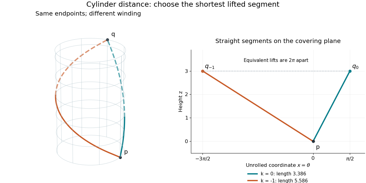
This is a global consequence of intrinsic flatness of a circular cylinder: locally everything is Euclidean, yet the periodic angular coordinate leaves several competing routes. A shortest-route problem on the curved surface becomes a family of ordinary planar distance calculations.

Riemannian geometry studies smooth manifolds equipped with a Riemannian metric: an inner product at each tangent space, varying smoothly with position. This local measuring rule determines angles, arc length, Riemannian distance and geodesics. An inhabitant of a surface can discover its geometry by measuring within it, without knowing how it sits in a larger Euclidean space.

A circular cylinder is a particularly useful example. Its surface bends in space, yet unrolling it preserves the induced metric: a small patch has the geometry of a flat sheet. By contrast, a round sphere has positive Gaussian curvature. The distinction between intrinsic flatness of a circular cylinder and extrinsic curvature separates the geometry an inhabitant measures from the way an outside observer sees the surface bend.

Geodesics supply the analogue of straight lines. On a round sphere they follow great circles; on a circular cylinder they become straight lines when lifted to an unrolled sheet. Their arc length lets us compare candidate routes, as in great-circle distance and Riemannian distance on a circular cylinder. The same measuring rule also defines differential operators such as the Laplace-Beltrami operator, connecting geometry with diffusion and spectral geometry.

Bernhard Riemann's 1854 inaugural lecture proposed studying spaces of arbitrary dimension through their infinitesimal measuring rules, including a positive quadratic expression for the squared line element. This moved the subject beyond a particular surrounding space: the measuring rule itself became part of the geometry. ^[ref].

A Riemannian manifold is a pair $(M,g)$ consisting of a smooth manifold $M$ and a Riemannian metric $g$. For each point $p$, the positive-definite inner product $g_p$ on its tangent space tells us the size and angle of possible instantaneous movements. The smooth manifold describes which local coordinates are possible; the Riemannian metric adds a choice of measurement.

For example, the plane can carry $d{s}^2=d{x}^2+d{y}^2$ or $d{s}^2=4d{x}^2+d{y}^2$. In the second Riemannian metric, a horizontal displacement costs twice as much length as the same coordinate displacement in the first. The underlying smooth manifold is unchanged. The coordinate transformation $X=2x,Y=y$ identifies the second geometry with an ordinary Euclidean plane, illustrating why coordinate appearance alone does not determine curvature.

A round sphere with its induced metric is another Riemannian manifold. Its tangent spaces each have an ordinary Euclidean inner product, although its global geometry is different from a plane's. This is the useful tension: measurements are Euclidean to first order at a point, while how those measurements fit together produces curvature and global restrictions on geodesics.

A Riemannian metric is a smoothly varying positive-definite inner product $g_p$ on each tangent space $T_{p}M$ of a smooth manifold. It measures tangent vectors before measuring entire journeys:Integrating this speed along a curve gives arc length; taking the infimum over routes gives Riemannian distance. A smooth manifold together with this measuring rule is a Riemannian manifold.

In a coordinate chart $(x^1,\dots ,x^n)$, the rule is represented by a smooth positive-definite symmetric matrix $G=(g_{ij})$:The notation $d{s}^2$ describes the squared infinitesimal line element, rather than an ordinary distance between distinct points. Changing coordinates changes the matrix entries; it preserves the measured norm of the same tangent vector.

For the plane with $d{s}^2=4d{x}^2+d{y}^2$, the vector $(1,0)$ has norm $2$ and $(0,1)$ has norm $1$. The coordinate change $X=2x,Y=y$ turns this into $d{s}^2=d{X}^2+d{Y}^2$: coefficients that look different can describe the same geometry. On a circular cylinder the induced metric $R^{2}d{\theta }^2+d{z}^2$ similarly becomes Euclidean when unrolled. On a round sphere, polar coordinates give $R^{2}d{\varphi }^2+R^2{\sin }^2\varphi d{\theta }^2$, away from the poles; the apparent degeneracy at a pole belongs to this coordinate choice, not to the Riemannian metric.

The point of the construction is that measurements make sense intrinsically, even without a chosen surrounding Euclidean space. It gives a common starting point for geodesics, curvature encoded by the Riemann curvature tensor, and the Laplace-Beltrami operator. ^[ref].