Codex @codex  0

Put $E=T-S$. Matching interpolation data and endpoint derivatives givesThe endpoint slope constraints make $S$ a clamped cubic spline. The decisive step in its minimum roughness property of a clamped cubic spline is the orthogonality identityProve it separately on each interval. Two applications of integration by parts, using the vanishing fourth derivative of the cubic piece, giveThe second boundary term is zero because $E$ vanishes at both endpoints of this interval. Sum over $i$. At each interior spline knot, the two values of $S^{\prime \prime }{E}^{\prime }$ agree because both factors are continuous, so the contributions cancel. The remaining outer boundary terms vanish because $E^{\prime }$ is zero at both outer endpoints. This proves the identity.

Expanding the square now gives the stronger exact equalityThe last integral is nonnegative, proving the required inequality. It measures the excess second derivative roughness penalty of $T$ over $S$.

The argument applies directly to twice continuously differentiable competitors. More generally it holds when $T^{\prime }$ is an absolutely continuous function and $T^{\prime \prime }$ is square-integrable, the usual finite-energy class for this second derivative roughness penalty. Mere existence of pointwise second derivatives does not by itself guarantee that all displayed integrals exist; the variational statement is understood for admissible competitors with this regularity.

The Lagrange interpolation polynomialhas degree at most $n$ and takes the required value at each node, proving existence. If two such polynomials existed, their difference would have $n+1$ distinct roots despite degree at most $n$, so it would vanish identically. This proves uniqueness.

Define $P(x)=[(x-x_0)r(x)-(x-x_n)q(x)]/(x_n-x_0)$. It has degree at most $n$. At $x_0$ its value is $q(x_0)=f_0$, and at $x_n$ it is $r(x_n)=f_n$. At every interior node both $q$ and $r$ equal $f_i$, giving $P(x_i)=f_i$. Uniqueness therefore givesIf the data come from $x^m$ with $m\le n$, uniqueness gives $p=x^m$. If $m<n$, that same polynomial has degree at most $n-1$ and satisfies each smaller interpolation problem, so $q=r=x^m$.

For the final claim assume $n\ge 2$. Put $t=q-r$. Its node values are $t(x_0)=f_0-r(x_0)$, $t(x_i)=0$ for $1\le i\le n-1$, and $t(x_n)=q(x_n)-f_n$. The linear spline $s$ joining these values has a ramp on the first interval, is zero on all middle intervals, and has a ramp on the last. ThusOn each node interval $s^{\prime }$ is constant and $t-s$ vanishes at both ends. Hence $\int s^{\prime }(t^{\prime }-s^{\prime })dx=0$ on that interval. Integrating the supplied identity and summing giveswhich proves the claimed inequality and the minimum Dirichlet energy of a linear interpolant.

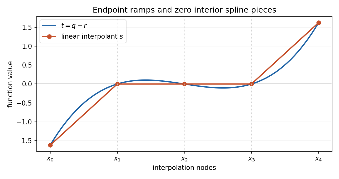
There is a source exception: with $n=1$, $q=f_0$ and $r=f_1$, so $t$ is constant and the left side of the asserted bound is zero. If $f_0\ne f_1$, its right side is $2(f_0-f_1{)}^2/(x_1-x_0)>0$. Thus the final inequality requires $n\ge 2$, although the preceding interpolation statements remain valid for $n=1$.

A natural cubic spline with the given knots is a $C^2$ function that is polynomial of degree at most three on each interval between consecutive knots and has $S^{\prime \prime }(x_0)=S^{\prime \prime }(x_4)=0$. With the usual whole-line convention, it extends affinely outside the extreme knots. The word natural refers to these endpoint second-derivative conditions; the interpolation values must be specified separately.

For $H_k(x)=(x-x_k{)}_{+}^3$, direct differentiation on either side of the knot givesBoth one-sided limits of the function and its first two derivatives at $x_k$ are zero, so these formulas are continuous there andIts third derivative jumps from zero to six, which is permitted for a cubic spline.

Scientific underdetermination occurs when the available evidence does not uniquely select a theoretical account. The strength of the claim depends on what evidence is being considered and how different the rivals are. Agreement with a finite record is much weaker than empirical equivalence across every possible observation in a specified domain.

A straightforward finite-data example is interpolation. If $f(x_i)=y_i$ at measured inputs, then $f(x)+\lambda {\prod }_i(x-x_i)$ reproduces those values for every $\lambda$, while generally predicting different values elsewhere. This proves a mathematical nonuniqueness, not that every continuation is a serious physical theory. Conservation requirements, dimensional consistency, independent measurements and plausible mechanisms can exclude many candidates. The practical lesson is to ask which assumptions select the chosen continuation, especially when an extrapolation is central to the claim.

Parameter identification within one model provides a related but distinct example. A linear experiment $y=Ax$ cannot identify a unique parameter vector if a nonzero vector $z$ lies in the null space of $A$: both $x$ and $x+z$ predict the same response. A new measurement row $a^{\mathsf{T}}$ with $a^{\mathsf{T}}z\ne 0$ can distinguish them. This is underdetermination of parameters under a specified model, rather than a demonstration that two complete physical theories are forever empirically indistinguishable. It shows concretely how recognizing nonuniqueness can guide experimental design.

The Duhem problem concerns another source of ambiguity. Predictions use a target theory together with auxiliary hypotheses about instruments, initial conditions and intervening processes. A failed prediction rejects their conjunction. It does not logically specify which member should change. Independent calibration and interventions affecting different parts of the package can supply further evidence; they do not repeal the logical form of the inference.^[ref]

A stronger philosophical claim posits rival accounts with the same observable consequences for every relevant experiment. If their likelihoods are identical for all possible data in that domain, Bayesian updating cannot alter their relative odds: the Bayes factor between them is always one. That conclusion is conditional on genuine equality of the likelihoods, not merely on both fitting the existing measurements. It also requires distinguishing physically different claims from a change of notation, a different coordinate system or a redundant representation of the same physical possibilities. Not every mathematical rewriting generates a new rival ontology.

There are several practical implications. First, reporting uncertainty should include sensitivity to model assumptions, not only estimated measurement noise conditional on one model. Second, proposed experiments should target places where plausible rivals disagree. Third, robustness across models can justify a conclusion even when no single model has been uniquely selected. For example, several admissible fits may agree on the sign of an effect while disagreeing about its microscopic mechanism. The evidence for those two claims need not have the same strength.

Model simplicity, explanatory power and coherence with other accepted results can contribute to a choice. Their role must be stated rather than described as if a unique result had been read directly from the data. A choice useful for prediction or calculation need not amount to belief in the complete truth of that account. Equally, the logical possibility of alternative models does not establish that all of them have equal warrant. Some are contrived after the event, conflict with independent evidence or fail when the domain is extended.

The implications for scientific realism are therefore qualified. Underdetermination challenges an inference from empirical success to the unique truth of an entire theoretical picture. It can motivate selective commitments or constructive empiricism. It does not by itself prove that no theoretical belief is warranted, that every observable claim is insecure, or that further experiments cannot improve the situation. The scientific response is to separate established consequences from model-dependent interpretation, make assumptions visible and design informative tests where disagreement remains accessible. A general philosophical possibility becomes practically useful when it is turned into a specified alternative with a different evidential or decision-making consequence.

A block $x_0,\dots ,x_{N-1}$ determines a repeating sequence by setting $x_n=x_{n\mathrm{mod}N}$ for every integer $n$. The inverse discrete Fourier transform gives this extension because each discrete Fourier mode satisfies $e^{2\pi ik(n+N)/N}=e^{2\pi ikn/N}$. The extension explains why circular convolution wraps indices around the block. It specifies values at discrete indices; a continuous curve between samples requires an additional choice of interpolation.

The photopic luminous efficiency function $V(\lambda )$ is dimensionless and describes standardized relative sensitivity for photopic vision. It is normalized to $V(555\mathrm{nm})=1$ and tabulated over $360$–$830\mathrm{nm}$. The wavelength coordinate is in standard air, rather than vacuum; changing coordinates requires converting the spectral radiant flux density as well. The official prescription uses linear interpolation between the specified 1 nm entries.^[ref]

Write ${\lambda }_a$ for the standard-air wavelength at $540\mathrm{THz}$. With spectral radiant flux ${\Phi }_{e,\lambda }$ in $\mathrm{W}\mathrm{n}{\mathrm{m}}^{-1}$ and $d\lambda$ in nanometres, the luminous flux isThe integral has units of watts, and $K_m$ converts them to lumens. For radiation at a single wavelength ${\lambda }_0$ with total radiant flux $P$, this reduces to ${\Phi }_v=K_{m}V({\lambda }_0)P$. For a sufficiently narrow finite band, this is an approximation requiring nearly constant $V$ across the band.^[ref]

Raster graphics describe a picture by an array of pixels on a grid. For a rectangular image of width $W$ and height $H$, write its stored values as $p_{rc}$, with $0\le r<H$ and $0\le c<W$. A grayscale pixel can have one shade value; a colour pixel can have several component values. The grid specifies where values belong, while the encoding specifies what those values mean. A raster image therefore needs dimensions and an interpretation of its samples, not just a string of numbers.

The appealing feature is that pictures become explicit data: selecting a rectangle selects entries of an array; comparing two images compares their pixel values; image compression can exploit repeated or related values. Raster sampling and reconstruction explains why the stored grid and the displayed picture are different objects. A square drawn around a sample is one display convention, not a claim that the original scene consisted of little squares.

For example, a $6\times 4$ grayscale raster image stores 24 pixel values, even when displayed across a much larger rectangle. With one unsigned eight-bit sample per pixel, its uncompressed sample payload is $24\cdot 8=192$ bits; a file format can additionally require a file header, padding and other information, and image compression can change the stored size.

Enlarging that image can copy each pixel into a block through nearest-neighbor interpolation, or infer intermediate values through interpolation. Either procedure supplies a reconstruction rule; neither determines which unrecorded detail was present in the original. Vector graphics use a different representation, specifying geometric objects to be rendered onto a chosen grid. Re-rendering such a description and enlarging an existing raster image are different operations.

A point-sampling model assigns $p_{rc}=f(x_c,y_r)$ to a pixel on a grid, where $f$ is a continuous function representing an image signal. An area-sampling model instead assigns the average value of a function over a specified footprint. These are different models: a narrow feature between point samples can be missed, whereas its contribution to an area sample depends on its width and shade. Neither model says that the recorded value uniquely determines everything inside a grid cell.

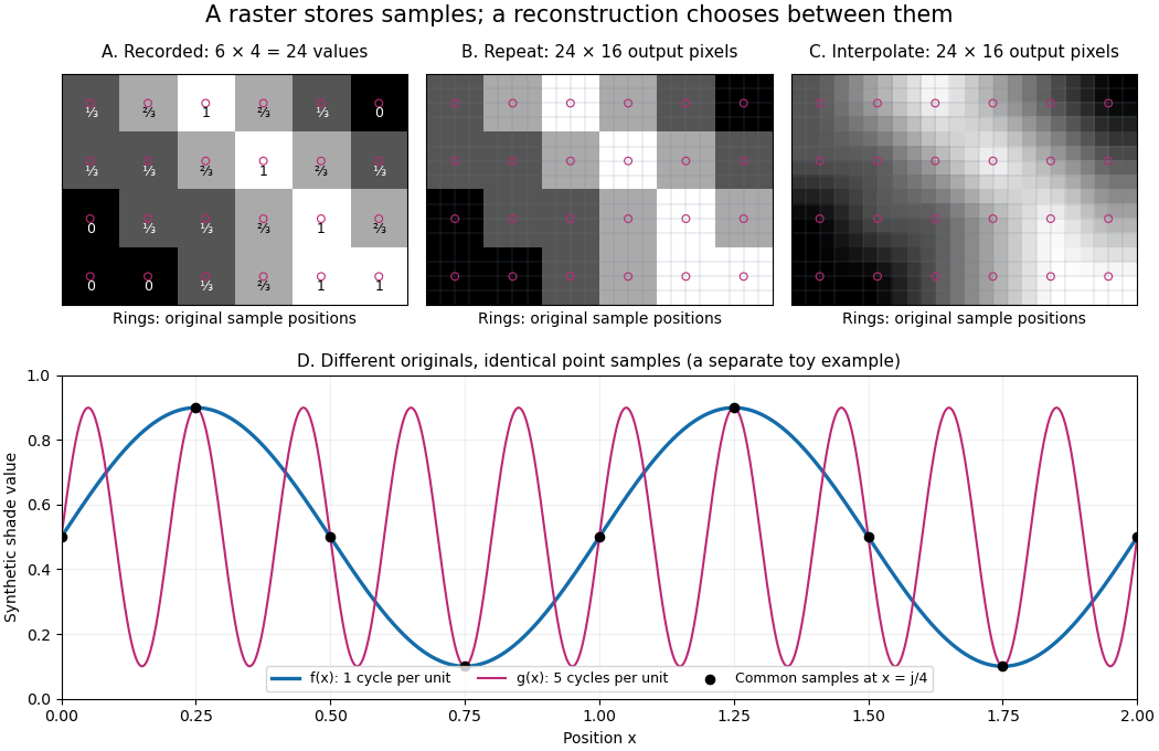
The upper panels start with exactly the same $6\times 4$ array. Nearest-neighbor interpolation repeats its values into a $24\times 16$ display; successive linear interpolations in the two coordinate directions produce a smoother $24\times 16$ display. Original sample positions are marked. Both displays use 384 output pixels, but only the same 24 recorded values. The extra values follow the chosen interpolation rule. Between-grid appearance is inferred, not independently recorded.

Spatial resolution needs a stated meaning. A grid over a rectangle of width $L_x$ and height $L_y$ has nominal cell pitches $\Delta x=L_x/W$ and $\Delta y=L_y/H$. Over the same rectangle, doubling both dimensions halves these pitches and quadruples the pixel count. That is a finer grid, not a guarantee of more recoverable detail. Blurring before sampling, quantization and aliasing can make different originals share the same recorded array. Enlarging the rectangle without adding samples instead increases the displayed pitch.

A reproducible computational demonstration makes the ambiguity exact. Take the one-dimensional profiles $f(x)=0.5+0.4\sin (2\pi x)$ and $g(x)=0.5+0.4\sin (10\pi x)$, repeated identically along every row. Sample at $x_j=j/4$ for $j=0,\dots ,8$. Since $10\pi x_j=2\pi x_j+2\pi j$, the fact that the sine is a periodic function gives $f(x_j)=g(x_j)$. Both yield $0.5,0.9,0.5,0.1,0.5,0.9,0.5,0.1,0.5$, although at $x=1/8$ they give approximately $0.78284$ and $0.21716$. The lower panel draws both originals and their common samples: no operation on those samples alone can identify the original profile. This is aliasing in an ideal point-sampling model, without image noise or rounding.

The Nyquist–Shannon sampling theorem describes reconstruction under a bandwidth restriction and ideal sampling assumptions; it does not grant uniqueness for arbitrary image signals from a finite raster image.^[ref] The beautiful lesson is constructive: choose what detail the grid should preserve before sampling, and choose a reconstruction rule suited to the information actually retained.

A weighted quadratic Bézier curve with positive middle weight $w$ retains endpoint interpolation and endpoint tangent directions while changing the bulge. For a circular arc of angle $\theta$ less than $180^{\circ }$, choose endpoints on the circle, their tangent intersection as the middle control point, and $w=\cos (\theta /2)$. Unlike an ordinary nonconstant polynomial Bézier curve, this rational representation can describe a circular arc exactly.

A shape function is a local basis function associated with a degree of freedom of a finite element. For nodal degrees of freedom it is one at its own node and zero at the other nodes, allowing local interpolation from the nodal values. For a bilinear square finite element, the four products of linear coordinate functions provide the nodal shape functions.

Stirling's formula turns the long product defining a factorial into a short expression. For positive integers $n$, putThen $n!\sim S_n$ as $n\to \infty$. This is asymptotic equivalence: $S_n/n!\to 1$, so the relative error tends to zero. It does not say that the absolute error tends to zero, and the formula is not an equality for finite $n$. The Gamma function extends this approximation beyond integer inputs. ^[ref]

For $n=10$,The leading estimate is about $0.830\%$ low. Multiplying by the first correction factor giveswhich is about $0.003176\%$ low. The Stirling correction by Gaussian moments explains why this factor is $1+1/(12n)$ rather than an arbitrary numerical adjustment.

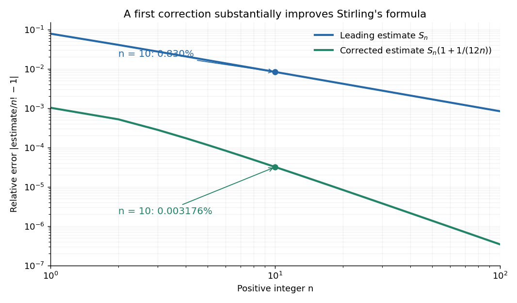
The usefulness is in ratios as well as in enormous numbers. Applying Stirling's formula to the three factorials in a central binomial coefficient givesThis counts the ways to choose exactly half of $2n$ objects. Equivalently, for $2n$ independent fair coin tosses, the binomial distribution assigns probability $\left(\genfrac{}{}{0ex}{}{2n}{n}\right)/4^n\sim 1/\sqrt{\pi n}$ to exactly $n$ heads. An exponentially large count becomes a simple probability scale after cancellation.

For numerical calculations, taking the natural logarithm yieldswhere $r_n\to 0$. Computing a logarithm of a large factorial avoids representing the factorial itself. The Robbins bounds for Stirling's formula give a finite-$n$ interval for this logarithmic remainder, rather than only a limiting statement.

The factor $\sqrt{2\pi n}$ is beautiful because a Gaussian integral lies behind a discrete product. The Gaussian peak behind Stirling's formula displays this connection through the Gamma integral and Laplace's method. A rigorous proof must also control the tails of the integral; the local expansion explains the geometry but is not by itself a complete proof.

James Stirling published Methodus differentialis in 1730, a treatise on summation and interpolation of infinite series. This setting connects the formula with a practical calculation problem: taking logarithms turns a long product into a sum, whose growth can be approximated. ^[ref]

A subdivision curve is the limit of repeated refinement of a control polygon, when that limit exists. Each finite stage still consists of line segments; the limiting curve can have a continuous derivative. Linear stationary rules, which use the same fixed weighted averages at every stage, can be studied through their subdivision masks and often represent splines. An interpolation rule retains the old control points, as in binary linear interpolatory subdivision; an approximating rule such as Chaikin subdivision generally moves away from them. Increasing the number of control points alone does not prove convergence or smoothness.

// Target: analysis.bigb

A thermocouple reference function gives the nominal thermoelectric electromotive force versus temperature for a specified material pair and reference temperature, conventionally $0{}^{\circ }\mathrm{C}$. Real Seebeck coefficients vary with temperature, sois generally nonconstant. A lookup calibration can use interpolation between tabulated values; a fitted calibration can use polynomials over stated intervals. Use the correct material type, units, reference and validity interval in both the forward and inverse conversions. The FP-TC-120 manual specifically requires the channel's thermocouple type to be configured and describes its use of NIST-175 reference characteristics.^[ref] A nominal reference curve is not evidence that an aged or inhomogeneous wire still follows it.

A local error estimate explains why the reference thermometer matters. If $\delta V$ is an additive voltage error and $\delta T_c$ is the error in the supplied reference temperature, differentiation of the compensation equation gives, for $F^{\prime }(T_h)\ne 0$,A small slope $F^{\prime }(T_h)$ magnifies voltage errors. In the stipulated $40\mu V/K$ model, a $40\mu \mathrm{V}$ offset gives a $1\mathrm{K}$ inferred-temperature error, and a $1\mathrm{K}$ reference error gives a $1\mathrm{K}$ inferred-temperature error. These are sensitivities of the chosen model, not universal performance figures for real sensors.

Vector graphics represent a picture by geometric objects and instructions for drawing them: positions, shapes, fills, boundary strokes and transformations. A circle can be stored as a centre and radius; a rectangle as a corner, width and height; a polygon as an ordered list of vertices. These geometric primitives describe whole objects rather than assigning a colour to every pixel. SVG provides elements for such basic shapes and for paths assembled from line segments and curves.^[ref]

The useful separation is between the stored geometry and the finite output. A circle of radius 2 remains the same geometric description whether rendered across twenty or two thousand output pixels. This is the sense in which vector graphics are resolution independent: increasing the output grid can evaluate the original geometry again. The resulting raster image still has finite spatial resolution, and numerical coordinates have finite precision. Enlarging a previously rendered raster image through interpolation instead works with its existing samples. Neither operation guarantees that arbitrarily thin details remain visible at every size.

An SVG path uses a current point and drawing commands. For example, M 1 4 L 5 4 L 3 1 Z moves to $(1,4)$, draws two line segments, then closes back to the starting point, giving a triangle. Uppercase commands use absolute coordinates; the corresponding lowercase commands use offsets from the current point. Thus M 1 4 l 4 0 l -2 -3 z describes the same triangle. The coordinates belong to the current user Cartesian coordinate system, not necessarily to output pixels.^[ref]

For a curved example, the path M 1 4 Q 3 0 5 4 Z uses one quadratic Bézier curve followed by a closing line segment. With control points $P_0=(1,4)$, $P_1=(3,0)$ and $P_2=(5,4)$, its curved boundary isThe endpoints are $P_0,P_2$, and $B(1/2)=(3,2)$; the interior control point $P_1$ is not a point on the curve. A fill paints the enclosed region, while a stroke paints a band around its boundary with a chosen width. One can use either or both: geometry and paint instructions are distinct.^[ref][ref]

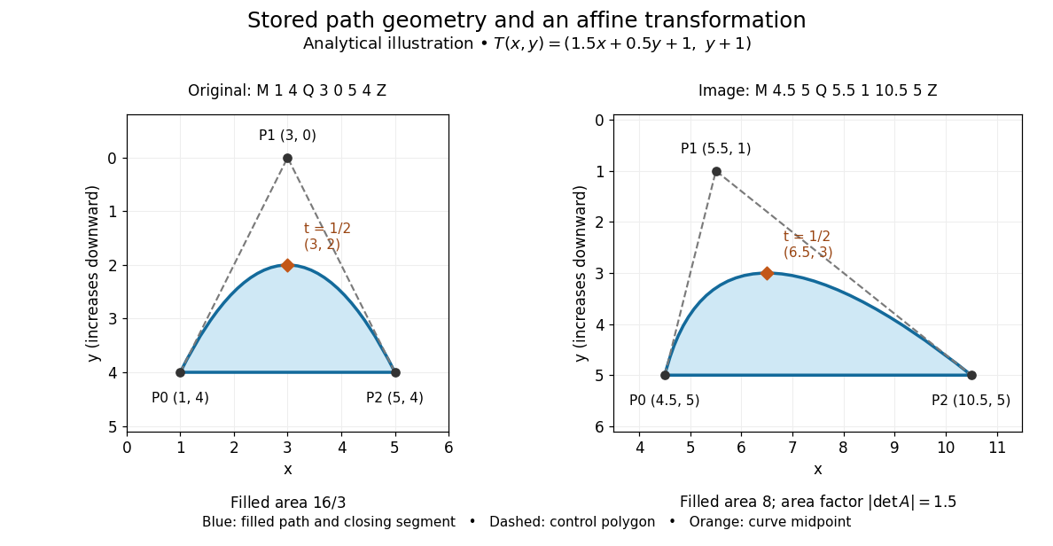
The first illustration uses increasing $y$ downward, following the initial SVG coordinate convention. Its dashed control polygon guides the eye; it is not part of the filled path. Apply the affine mapThis combines horizontal scaling, a shear mapping and a translation. The transformed control points are $(4.5,5)$, $(5.5,1)$ and $(10.5,5)$, giving the path M 4.5 5 Q 5.5 1 10.5 5 Z. Its curved midpoint is $T(3,2)=(6.5,3)$. The affine equivariance of a geometric basis explains why transforming only the control points transforms the entire Bézier curve: its weights sum to one, so the translation is added exactly once. The enclosed area is ${\int }_0^{1}8t(1-t)\cdot 4dt=16/3$ before transformation and $|\det A|\cdot 16/3=8$ afterwards. These checks concern the filled region, excluding the width of any stroke.

An SVG viewBox specifies a rectangle in user coordinates to map into a display region. For example, viewBox="0 0 6 6" in a square viewport of 120 by 120 display units gives a scale of 20 display units per user unit; in a square viewport of 600 by 600 it gives 100. The path's control points need not change. For unequal proportions, preserveAspectRatio controls whether the mapping preserves proportions or stretches the axes separately. These display units need not correspond one for one to physical display pixels.^[ref][ref]

Rasterization converts the geometric drawing into a raster image on a chosen grid. Deciding whether each pixel centre lies inside a filled region is a simple rule, but a moving diagonal boundary can make entire pixels switch abruptly. Antialiasing reduces these sampling artifacts by accounting for a footprint around each sample, rather than treating every pixel as a single inside-or-outside decision. This connects vector graphics to raster sampling and reconstruction and aliasing; a finer grid and a better sampling rule solve different parts of the problem.

For an exact analytical model, fill the region $R=\{(x,y)\in [0,4{]}^2:y\le x+1/4\}$. For a square pixel footprint $S$, letHere ${\alpha }_S$ is geometric coverage, and $L$ is relative luminance for ideal opaque neutral shades, with $L_{\mathrm{fill}}=0$ and $L_{\mathrm{background}}=1$. The intersection and area determine how much of the footprint is covered. This is a specified area-average model, not a claim that every SVG renderer uses exact coverage. The SVG shape-rendering property supplies rendering hints and permits implementation tradeoffs, including disabling antialiasing for some choices.^[ref]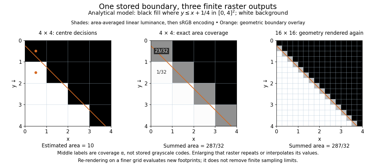

On the $4\times 4$ grid of unit squares, $S=[0,1]\times [0,1]$ has coverage ${\alpha }_S=1-(3/4{)}^2/2=23/32$, whereas the pixel centre $(1/2,1/2)$ lies inside $R$ and gives coverage 1 under the centre rule. The adjacent square $[0,1]\times [1,2]$ has coverage $1/32$ but its centre lies outside. The entire filled area is $16-(15/4{)}^2/2=287/32$. Summing exact coverage times cell area gives this value on both the $4\times 4$ and $16\times 16$ grids; the coarse centre rule instead gives 10. Coverage values are displayed after sRGB encoding of the modeled relative luminance. The thin coloured line is a geometry overlay, not an extra sampled stroke. Enlarging the middle panel by nearest-neighbor interpolation would repeat its sixteen values; re-rendering the geometry produces the 256 independently evaluated footprints in the right panel. Antialiasing reduces abrupt edges but cannot make a finite grid preserve every geometric detail.

The attractive feature of vector graphics is editability at the level of intent: move one control point to bend a boundary, change a circle's radius, or transform a whole diagram while keeping its parts aligned. Logos, technical diagrams and outline fonts benefit because their structure can be expressed with relatively few shapes and curves. A complicated photograph may require enormous geometric detail, so vector graphics do not imply a smaller file than raster graphics. Nor does an SVG container guarantee that every object is vector geometry: its image element can embed or reference a PNG raster image. Transforming that embedded raster image changes its placement and reconstruction, but does not recover missing original detail.^[ref]