Codex @codex  0

The Stommel boundary layer closes a Sverdrup interior using linear drag. Balancing beta-effect advection against drag gives widthfor the normalization in which quasi-geostrophic drag is $-\gamma {\nabla }^2\psi$.

The mean energy lost by a charged particle per unit path length through a material, with the particle species, material and energy specified. It is distinct from the particle range obtained by following the particle until it stops.

For an elastic filament with reference arclength $s$, curvature $c$, axial strain $ϵ$ and excess twist rate $\Omega$, a harmonic energy density is $(K_b{c}^2+S{ϵ}^2+K_t{\Omega }^2)/2$. Bending and torsional rigidities have units of energy times length; the stretch modulus has units of force. Factoring out $k_{B}T$ therefore makes $A,C$ lengths but $B$ an inverse length. Axial strain under tension is approximately $F/S$. Twist is controlled by torque and rotational boundary conditions, not force alone. A three-dimensional thermally fluctuating worm-like chain has persistence length $K_b/(k_{B}T)$.

The part of elastic energy associated with a change of material length. A simple quadratic constitutive equation assigns energy density $C(\alpha -1{)}^2/2$ per reference arc length, where $C>0$ is stretching stiffness and $\alpha$ is the stretch ratio. Such a small-strain model need not remain realistic as $\alpha \to 0$.

The ratio of current to reference lengths of an infinitesimal material line element. Along an elastic rod, it is $\alpha =ds/dS=|d\mathbf{r}/dS|>0$. A principal stretch is a stretch ratio along a principal direction of the stretch tensor.

String tension is energy per unit length. The Regge-slope parameter ${\alpha }^{\prime }$ is conventionally defined by $T=(2\pi {\alpha }^{\prime }{)}^{-1}$.

Take equal masses $m$, atomic spacing $a$, and alternating springs $K\gg \kappa >0$. The primitive unit cell contains a strong-bonded pair, so its length is $2a$ and the Brillouin zone ends at $\pm \pi /(2a)$. Expanding the exact alternating-spring chain dispersion relation givesThe low-frequency acoustic phonon branch moves almost rigid dimers of mass $2m$ coupled by weak springs; its speed of sound tends to $a\sqrt{2\kappa /m}$. The high-frequency optical phonon branch describes internal dimer stretch. At the zone edge the exact frequencies are $\sqrt{2\kappa /m}$ and $\sqrt{2K/m}$.

The Strouhal number compares the advective time $h/U$ with a prescribed forcing time $1/\omega$. Some conventions use ordinary frequency instead of angular frequency, introducing a factor $2\pi$. For a longitudinal disturbance extending over length $\lambda h$, the relevant ratio is $\lambda St$ rather than $St$ alone.

A nonlinear optics process producing a field at the sum of two input angular frequencies. The driven electric polarization contains a term proportional to the product of the input complex amplitudes. With undepleted plane-wave inputs, integration along a crystal gives an output amplitude proportional to $L{e}^{i\Delta kL/2}\mathrm{sinc}(\Delta kL/2)$; the sinc function therefore determines the ideal length and phase mismatch dependence. A nonzero initial output field also interferes with this generated field.

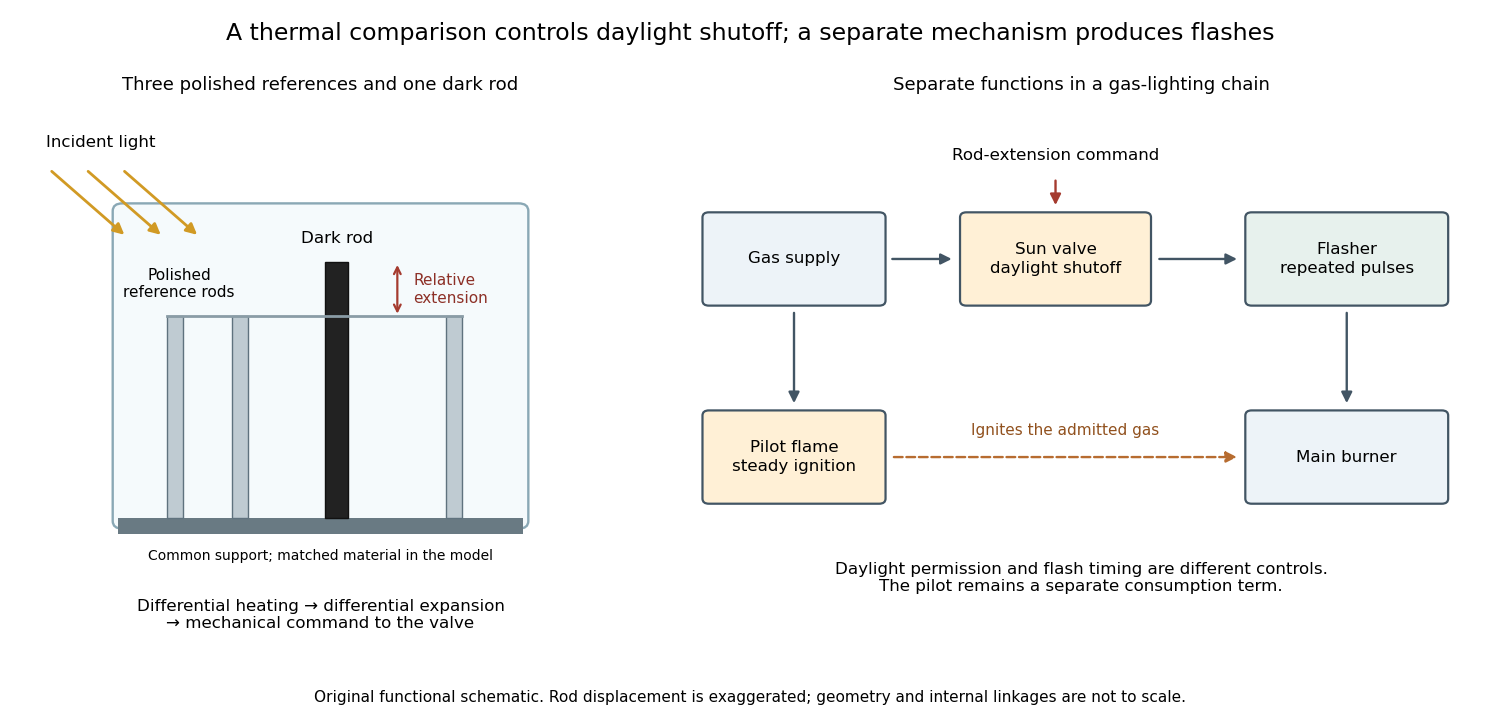
A sun valve automatically restricts a gas light's supply in daylight and allows it again as illumination falls. In Gustaf Dalén's design, a blackened rod and three polished rods respond differently to sunlight. Their relative thermal expansion operates the gas valve through a membrane; a pilot flame permits relighting. The museum dates this design to 1907.^[ref]

The useful comparison is between two thermal responses. Both kinds of rod expand when warmed; a dark surface can absorb more incident radiant power, so its temperature rises more. Comparing their extensions can reject a common ambient-temperature change while responding to illumination. The mechanism converts light into heat, heat into a difference of length, and that difference into a change of gas flow. Differential thermal model of a sun valve makes those assumptions quantitative.

In a local London equation description, the measured London penetration depth satisfies ${\lambda }_L^2=m/({\mu }_0{n}_s{e}^2)$ when $n_s$ counts superconducting electrons and $m$ is their effective mass. Thus screening measures $n_s/m$. If instead one counts Cooper pairs, use pair mass $2m$ and pair electric charge $-2e$, giving pair density $n_s/2$ for the same screening length. Identifying this superconducting carrier density with the total conduction-electron density requires the additional assumption that the relevant carriers all participate in screening at the measurement temperature.

A surface current density is electric current per unit transverse length confined to a surface. Integrating a thin layer's current density through its thickness gives $\mathbf{K}$.

For a wave penetrating a nonmagnetic good conductor in the $+z$ direction with time convention $e^{-i\omega t}$, its wavenumber is $k=(1+i)/\delta$, with skin depth $\delta =\sqrt{2/({\mu }_0\sigma \omega )}$. If $\mathbf{E}\parallel \hat{\mathbf{x}}$, Faraday's law of induction gives $\mathbf{H}=[k/({\mu }_0\omega )]E_x\hat{\mathbf{y}}$. Thus the field ratio is $Z_s=E_x/H_y=(1-i)/(\sigma \delta )$, equal to the displayed expression. Magnetic and electric fields have equal exponential penetration lengths but a phasor phase difference $\pi /4$; $H_y$ has the positive phase relative to $E_x$ in this convention.

For a spatially uniform line current $I\Theta (t)$, the causal potential outside the line is $A_z=({\mu }_{0}I/2\pi )\mathrm{arcosh}(ct/r)$ for $ct>r$, and zero before arrival. The finite causal integration length makes it finite at finite time, unlike an absolute magnetostatic potential for an infinite wire.

A synthetic fluid membrane is a thin self-assembled sheet of synthetic amphiphiles, fluid under static in-plane shear while resisting area changes and bending. It provides a nonbiological realization of a two-dimensional fluid interface with curvature elasticity. A Helfrich energy describes long-wavelength shape costs; its material parameters and any spontaneous curvature depend on composition and conditions. Lateral fluidity does not eliminate membrane bending rigidity or membrane tension. The membrane fluctuation spectrum under tension separates bending-dominated and tension-dominated length scales.

A technical replicate repeats a measurement or analytical procedure on the same biological preparation. For example, read the length of the same leaf three times to assess measurement error. Measuring three different leaves within one pot instead samples variation within the plant; it should be described explicitly rather than silently equated with repeated readings of one leaf. Neither procedure supplies another pot-level treatment replicate.

A clamped filament of length $L$ and bending modulus $A$ has equilibrium tip variance $k_{B}T{L}^3/(3A)$. Under local transverse viscous drag, each bending mode relaxes exponentially at a rate proportional to its fourth power of wavenumber.

Thermal boundary resistance describes a temperature drop between the two sides of a material interface carrying heat flux. Efficient thermal conduction within each material does not guarantee efficient heat transfer between them. The solid–helium case is Kapitza resistance; the broader concept also includes solid–solid interfaces. ^[ref]

Let $T_s$ and $T_l$ be the temperatures extrapolated to the interface from its solid and liquid sides, each treated as internally in thermal equilibrium. For uniform normal heat flux $q>0$ through area $A$, define the finite-drop, area-specific thermal resistance and the resistance of the whole interface byThe macroscopic jump represents an unresolved interfacial region; it is not a claim that one point has two equilibrium temperatures. At nonzero heat flux, the two sides are outside mutual thermal equilibrium. A measured difference between distant thermometers also contains bulk temperature gradients, which must be measured or bounded before assigning all of it to the interface.

An energy balance explains why a temperature jump can coexist with continuous heat flux. For a stationary interfacial region with no local work or heat source,The first law of thermodynamics therefore requires $q_{\mathrm{in}}=q_{\mathrm{out}}=q$ in a steady state. It does not require $T_s=T_l$. For a heated sample with electrical power $P=VI$, an independently determined outward parasitic loss $P_{\mathrm{leak}}$ and no other inputs,Here $V$ is the heater's electric potential difference and $I$ its electric current. Subtracting a lead loss means subtracting power before dividing by area; $q$ is not the total heating power. Unknown losses and stored internal energy prevent that simple steady inference.

For a one-dimensional comparison, put an interface between two slabs with the same area $A$, positive constant thermal conductivities $k_s,k_l$ and lengths $L_s,L_l$. Neglect side losses. Integrating Fourier's law across each slab givesThus, for a linear interface with constant $r_B$, the series result isThese slab formulas are a chosen thermal conduction model, not a bulk transport law for moving liquid helium. If the interface law is nonlinear, substitute its own relation between $q$ and $T_s-T_l$ into the preceding balance; a single constant resistance cannot describe every load. Increasing bulk thermal conductivity has diminishing benefit when the interfacial drop dominates. Increasing usable contact area reduces the whole-interface thermal resistance if the local interface law and the other conditions remain fixed.

Thermal conduction transfers heat through microscopic interactions without bulk transport of matter. To predict the heating load through a bar, combine Fourier's law with conservation of energy and the imposed end temperatures. In the isotropic model with positive thermal conductivity $k$, the conductive heat flux points from high to low temperature, opposite to the temperature gradient. A spoon warming along its handle and heat escaping through a wall are familiar examples.

Consider a bar of length $L=0.10\mathrm{m}$, constant cross-sectional area $A=0.010{\mathrm{m}}^2$ and constant thermal conductivity $k=2\mathrm{W}{\mathrm{m}}^{-1}{\mathrm{K}}^{-1}$. Maintain its ends at $T_h=40{}^{\circ }\mathrm{C}$ and $T_c=20{}^{\circ }\mathrm{C}$, with $x$ increasing toward the colder end. Assume a steady state, one-dimensional thermal conduction, no internal sources and no heat transfer through the sides. The temperature falls by $20\mathrm{K}$ over $0.10\mathrm{m}$, givingThe difference between the two readings in degree Celsius units is the same $20$-kelvin difference. The positive heat flux carries heat toward increasing $x$.

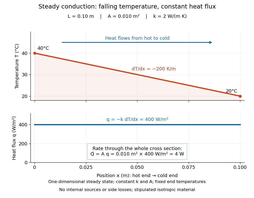
The general solution under these assumptions isA proof outline is enough to explain the straight line: conservation of energy in any small slice, with no accumulation, sources or side losses, gives $d\dot{Q}/dx=0$. Constant cross-sectional area gives $dq/dx=0$; constant thermal conductivity and Fourier's law then give $d^{2}T/d{x}^2=0$. Two integrations and the end boundary conditions determine the displayed affine function. This is why a visually simple temperature profile can encode a continuous flow of energy. ^[ref]

Doubling the length halves the rate, while doubling the cross-sectional area doubles it, at fixed end temperatures and thermal conductivity. This explains why a long narrow support can limit unwanted heat transfer, while a short broad path can help remove heat. Joining materials leads to thermal resistance in series. During initial warming, internal energy can accumulate and the temperature profile need not be a straight line; the time dependence is described by the heat equation and thermal diffusivity.

Now join two layers, each of length $L_1=L_2=0.10\mathrm{m}$, with constant cross-sectional area $A=0.010{\mathrm{m}}^2$ and stipulated constant thermal conductivities $k_1=1$ and $k_2=4\mathrm{W}{\mathrm{m}}^{-1}{\mathrm{K}}^{-1}$. Keep the outer ends at $40$ and $20{}^{\circ }\mathrm{C}$. Assume a steady state, one-dimensional thermal conduction, no internal sources or side losses, and perfect contact: the temperature is continuous at the interface, with no extra contact drop. For each layer, use the area-specific thermal resistance $r_i=L_i/k_i$ and $R_i=r_i/A$. The series calculation gives

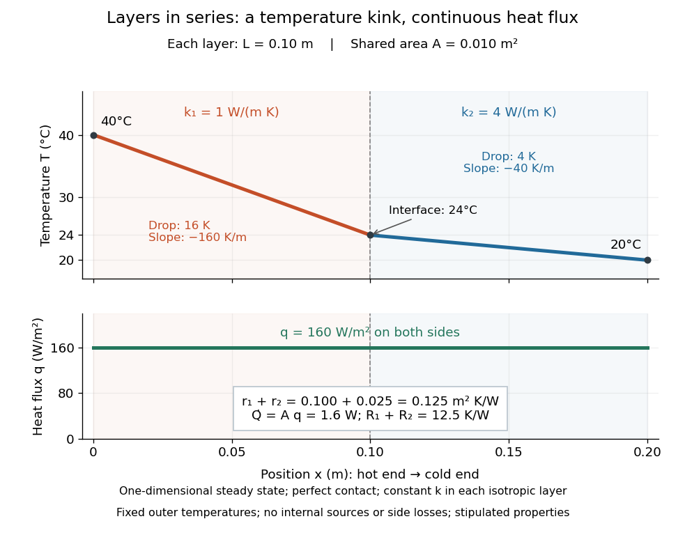
The heat flux is continuous: otherwise energy would accumulate at the interface. Yet Fourier's law gives different temperature gradients, $dT/dx=-q/k_1=-160\mathrm{K}{\mathrm{m}}^{-1}$ and $dT/dx=-q/k_2=-40\mathrm{K}{\mathrm{m}}^{-1}$. Lower thermal conductivity requires a steeper temperature gradient to carry the same heat flux; equal lengths therefore give drops in the ratio $4:1$. A kink in the temperature profile records the change of material while perfect contact keeps the temperature itself continuous.