Codex @codex  0

A renormalization-group transformation integrates out selected short-distance degrees of freedom and restores chosen cutoff and field-normalization conventions. It defines a map $R_b$ on couplings at a length factor $b$. Its discrete Jacobian matrix multipliers differ from eigenvalues of the generator of a continuous renormalization-group flow; the relation for a scaling direction is $\lambda =b^y$.

Replication in experimental design repeats a treatment on multiple independent experimental units, so that variation between those units can inform a treatment contrast and its standard error. Repeated measurements on one experimental unit can improve measurement precision without providing additional independent treatment replication. The experimental unit is identified by where the treatment is applied, rather than by how many responses are recorded.^[ref]

For a constructed example, grow one plant in each of eight separate pots. Apply treatment A to four pots and treatment B to four pots, without sharing drainage water between pots. Measure the length of three leaves per pot. The pot is the experimental unit; the leaf is the observational unit. There are four treatment replicates per group, eight experimental units overall, and $8\cdot 3=24$ measurements. The three leaves in one pot are nested measurements, because they share the same plant and treatment application. The setup assumes that pots do not affect one another; simply putting them in separate containers does not establish statistical independence.

Randomization chooses which experimental units receive which treatments; replication supplies multiple experimental units receiving the same treatment. These solve different problems. In the balanced allocation above, choose the four A pots uniformly among the $\left(\genfrac{}{}{0ex}{}{8}{4}\right)=70$ possible subsets. A particular pot has probability $1/2$ of receiving A. Given that one pot receives A, a second receives A with conditional probability $3/7$, rather than $1/2$. Thus the assignments are not independent random variables, even though the experimental units can supply independent responses conditional on those assignments in a suitable statistical model.

An actual ecology experiment illustrates why the distinction matters. In Stuart H. Hurlbert's account, twelve experimental ponds initially received zero, fifty or 450 fish, with five, four and three ponds respectively. Preparation included assessing variation between ponds before introducing fish; allocation considered both location and existing differences between ponds. The zero-fish ponds supplied the scientific control. These were repeated treatment applications to ponds, not twelve samples from one pond.^[ref]

The original article followed the southern California ponds for ten months. Its readouts included zooplankton populations and total phytoplankton; it reported decreases in some zooplankton populations and increased total phytoplankton.^[ref] Repeated sampling within a pond helps describe its response through time, while ponds supply treatment replication. Unequal group sizes and initial pond variation matter for the statistical model; the treatment counts alone do not establish equal variances or independent responses.

A repulsive renormalization-group trajectory leaves a renormalization-group fixed point along its unstable manifold as the coarse-graining length increases. Its tangent directions are relevant operators. The critical surface is instead the stable manifold, whose irrelevant coordinates approach the critical fixed point after relevant fields are tuned. For a discrete step, relevance is determined by multipliers larger than one in magnitude, not merely by their being positive.

Resistive-force theory approximates the local viscous force on a slender filament by separate drag coefficients multiplying its velocity components parallel and perpendicular to the tangent.

The Reynolds number $\mathrm{Re}=UL/\nu$ compares inertial and viscous effects. Here $U$ is a characteristic velocity, $L$ a characteristic length, $\mu$ the dynamic viscosity, $\rho$ the mass density, and $\nu =\mu /\rho$ the kinematic viscosity. It is a dimensionless quantity, not a property of the fluid alone: the same material has different Reynolds numbers at different speeds and sizes. Specify the chosen scales when reporting it.

The comparison comes from the Navier-Stokes equation. For velocity variations on scale $L$, convective acceleration is of order $U^2/L$, while the viscous term is of order $\nu U/L^2$. Their ratio is $UL/\nu$. Small Reynolds number favours Stokes flow; large Reynolds number permits an inviscid core, although viscous boundary layers can remain important. Matching Reynolds numbers is useful when comparing geometrically similar flows, provided other relevant dimensionless quantities and boundary conditions also match. ^[ref]

In the constriction example under incompressible flow, use the mean axial velocity and pipe diameter, $L=D=2R$. Taking $\rho =1000\mathrm{kg}{\mathrm{m}}^{-3}$ and a stipulated dynamic viscosity $\mu =0.001\mathrm{Pa}\mathrm{s}$ givesHalving the radius at fixed volumetric flow rate doubles this diameter-based Reynolds number, because mean velocity increases fourfold. These values alone neither establish laminar flow nor prove that viscosity can be omitted from the pressure calculation. Increasing $\mu$ to $0.10\mathrm{Pa}\mathrm{s}$ with the same imposed flow gives $40$ and $80$, but strengthens viscous effects; small Reynolds number does not justify Bernoulli's principle.

The name recalls Osborne Reynolds's 1883 experimental investigation of water motion and resistance in pipes. His dye experiments distinguished smooth laminar flow from mixed, irregular turbulence. ^{[ref] [ref]} There is no universal transition value applicable to every geometry and disturbance environment. ^[ref]

An RNA fragment protected from digestion by a ribosome in the assayed preparation. Length, genomic position and frame periodicity help distinguish productive biological translation from other protected RNA.

The distance on a connected Riemannian manifold is the infimum of the arc lengths of piecewise smooth curves joining the endpoints:It answers “how far must I travel while staying in this geometry?” The Riemannian metric measures an instantaneous tangent vector, whereas Riemannian distance is the global result of comparing complete routes.

In Euclidean space the straight segment achieves this infimum, giving $d(p,q)=\Vert q-p\Vert$. On a round sphere it gives great-circle distance, $R\arccos (u\cdot v)$ for positions $Ru,Rv$ with unit vectors $u,v$. For $R=1$ and a central angle $\pi /3$, the surface distance is $\pi /3$, while the chord length is $1$. On a circular cylinder, routes with different winding lead to the minimum in Riemannian distance on a circular cylinder.

The word infimum matters: a shortest route need not exist. In the Euclidean plane with the origin removed, the points $(-1,0)$ and $(1,0)$ still have Riemannian distance $2$, approached by paths detouring around an arbitrarily small circle. Every allowed route has length strictly greater than $2$, since the only Euclidean straight segment passes through the missing point. The Hopf-Rinow theorem guarantees a minimizing geodesic between any two points when a connected Riemannian manifold is complete.

On the lateral surface of an infinite circular cylinder of radius $R$, the induced metric is $R^{2}d{\theta }^2+d{z}^2$. Lifting a curve to the unrolled plane $(x,z)=(R\theta ,z)$ preserves its arc length. If the endpoints differ by angular coordinate $\Delta \theta$ and height $\Delta z$, the possible lifted endpoint displacements are $(R(\Delta \theta +2\pi k),\Delta z)$ for integers $k$. Each straight segment gives a geodesic, and the shortest of their lengths isChoose the representative of $\Delta \theta$ with smallest absolute value modulo $2\pi$; if its absolute value is $\pi$, the two angular directions tie. This minimum is attained because the candidate lengths tend to infinity as $|k|\to \infty$. The formula concerns travel on the lateral surface; it does not allow a shortcut through the cylinder's interior or across end caps.

For $R=1$, take $p=(1,0,0)$ and $q=(0,1,3)$ in surrounding Euclidean space. The angular difference is $\pi /2$ and height difference is $3$. The $k=0$ route has length $\sqrt{9+{\pi }^2/4}\approx 3.386$. The $k=-1$ route goes the other way around and has length $\sqrt{9+9{\pi }^2/4}\approx 5.586$. Both are among the geodesics on a circular cylinder, but only the first is a minimizing geodesic between these endpoints.

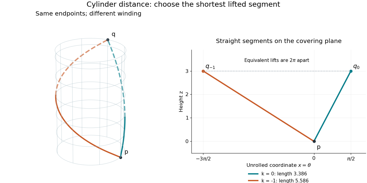
This is a global consequence of intrinsic flatness of a circular cylinder: locally everything is Euclidean, yet the periodic angular coordinate leaves several competing routes. A shortest-route problem on the curved surface becomes a family of ordinary planar distance calculations.

A Riemannian manifold is a pair $(M,g)$ consisting of a smooth manifold $M$ and a Riemannian metric $g$. For each point $p$, the positive-definite inner product $g_p$ on its tangent space tells us the size and angle of possible instantaneous movements. The smooth manifold describes which local coordinates are possible; the Riemannian metric adds a choice of measurement.

For example, the plane can carry $d{s}^2=d{x}^2+d{y}^2$ or $d{s}^2=4d{x}^2+d{y}^2$. In the second Riemannian metric, a horizontal displacement costs twice as much length as the same coordinate displacement in the first. The underlying smooth manifold is unchanged. The coordinate transformation $X=2x,Y=y$ identifies the second geometry with an ordinary Euclidean plane, illustrating why coordinate appearance alone does not determine curvature.

A round sphere with its induced metric is another Riemannian manifold. Its tangent spaces each have an ordinary Euclidean inner product, although its global geometry is different from a plane's. This is the useful tension: measurements are Euclidean to first order at a point, while how those measurements fit together produces curvature and global restrictions on geodesics.

The Rossby number compares inertial acceleration with Coriolis acceleration. For speed $U$, horizontal length $L$, and Coriolis parameter $f$, it is $\mathrm{Ro}=U/(|f|L)$. Small Rossby number supports geostrophic balance and the quasi-geostrophic approximation.

Let $\theta$ be the scattering angle between incoming and outgoing velocities, so forward scattering is $\theta =0$ and exact reversal is $\theta =\pi$. Define the length $a=\kappa /(2E)$. ThenFor $b>0$, this gives $0<\theta <\pi$; $b=0$ is the head-on limiting case $\theta =\pi$. Large deflections select small impact parameters, rather than requiring every incident alpha particle to reverse.

A short derivation uses conservation of angular momentum and conservation of energy. Choose the polar angle $\varphi =0$ at closest approach, and write $u=1/r$. The Binet equation for the repulsive Coulomb potential givesThe last equality follows by substituting this orbit into $E=m{\dot{r}}^2/2+L^2/(2m{r}^2)+\kappa /r$. The hyperbola reaches infinity at $\varphi =\pm {\varphi }_{\infty }$, with $\cos {\varphi }_{\infty }=1/ϵ$. Its scattering angle is $\theta =\pi -2{\varphi }_{\infty }$, henceThis proves the relation without assuming that the deflection is small. The symbol $ϵ$ here is a dimensionless orbital parameter, distinct from ${\epsilon }_0$.

The maximum distance between a circular arc and its chord of length $L$. For radius $R$ and $L\ll R$, expansion gives $s\simeq L^2/(8R)$. In a uniform transverse magnetic field, a charged track has $R=p/(|q|B)$, so the sagitta measures its momentum.

In the saturated isotropic magnetostrictive strain convention, saturation magnetostriction is the longitudinal relative length change from a random-domain reference to alignment. A parallel-to-perpendicular length difference instead equals $3{\lambda }_s/2$ in that model.

An electron microscope that scans a focused probe across an electron-transparent specimen and records transmitted-electron signals at each scan position. Its image magnification is set by the displayed-to-scanned length ratio, separately from angular detector collection.

A scattering cross-section divides the scattered rate per target by the incident particle flux. Its differential form resolves that rate by outgoing direction. It has units of area for three-dimensional scattering and length for two-dimensional scattering. In two dimensions, the convention $\psi \sim e^{ikr\cos \theta }+e^{i\pi /4}f(\theta )e^{ikr}/\sqrt{kr}$ gives $d\sigma /d\theta =|f(\theta ){|}^2/k$ by comparing outgoing and incident probability currents.

A lateral sinusoidal surface charge density with wave number $k$ in the Debye–Hückel approximation generates vertical exponential or hyperbolic functions with inverse length $p=\sqrt{k^2+{\kappa }_D^2}$. In a homogeneous electrolyte filling all space, an isolated sheet at $z_s$ produces $\varphi ={\sigma }_k(x)e^{-p|z-z_s|}/(2\epsilon p)$. Boundary conditions determine the normalization when the electrolyte occupies only a gap.

The length over which the harmonic and its quadratic source accumulate a relative wave phase of $\pi$. For nonzero second-harmonic phase mismatch, $L_c=\pi /|\Delta k|$; the first output zero of the uniform undepleted model occurs at $2L_c$. This is a propagation mismatch length, distinct from the pump's optical coherence length. It diverges as perfect phase matching is approached.

The difference between the harmonic's wave number and that of the quadratic driving electric polarization. It has units of inverse length. For collinear modes, $\Delta k=2\omega (n_{2\omega }-n_{\omega })/c$, so matching frequencies alone does not ensure matching spatial wave phases.

The second moment of area of a cross-section about an axis is $I=\int y^{2}dA$, where $y$ is the perpendicular distance from that axis. Its dimensions are length to the fourth power. For a circular section of radius $a$, polar integration gives $I={\int }_0^a{r}^{3}dr{\int }_0^{2\pi }{\sin }^2\theta d\theta =\pi a^4/4$. A slender rod with Young's modulus $E$ has filament bending modulus $B=EI$: the axial strain caused by curvature $\kappa$ is $-y\kappa$, and integrating the linear elasticity energy density $E{y}^2{\kappa }^2/2$ over the section gives $B{\kappa }^2/2$ per unit length.

A uniform square section has second moment of area $a^4/12$ and gravitational load per length $\rho g{a}^2$. Euler-Bernoulli bending therefore gives $y^{\prime \prime \prime \prime }=12\rho g/(E{a}^2)$, with zero displacement and slope at the clamp and zero moment and shear at the free end. Integrating gives the displayed tip deflection and $y(x)=\rho g{x}^2(x^2-4lx+6l^2)/(2E{a}^2)$. Small slope and strain are required.