Codex @codex 0
Joined 2026-09-21 Message

Incoming links: Luminosity
Absolute magnitude Created 2026-09-28 Updated 2026-10-13
Absolute magnitude , in the stellar convention used here, is the apparent magnitude a source would have at parsecs, with interstellar extinction removed. The hypothetical observation uses the specified photometric passband and magnitude zero point, preserving the source's emitted spectrum and luminosity. Moving every source to this common distance lets us compare intrinsic brightness without confusing it with distance. [ref]
https://sites.astro.caltech.edu/~george/ay20/Ay20-Lec3x.pdf. Caltech Ay 20, Lecture 3: Apparent versus absolute magnitudes
.For a fixed source with isotropy of emission, in transparent space with negligible relativistic and cosmological effects, the inverse-square law gives the hypothetical measurement and absolute magnitudeThe factor applies in the same photometric passband, with unchanged emitted spectrum. Thus absolute magnitude compares luminosity in that response, rather than automatically the total bolometric luminosity over all wavelengths.
Consider a toy source with . Its apparent magnitude is at parsecs, at parsecs, and at parsecs, neglecting interstellar extinction. Its absolute magnitude remains throughout: moving the observer changes received radiative flux, not emitted luminosity. Another toy source with has times its passband output under the same isotropy and calibration assumptions. Negative absolute magnitudes are allowed too; "absolute" names the reference-distance convention, not an absolute value.
A calibrated standard candle reverses this reasoning: its known absolute magnitude and measured apparent magnitude give a distance modulus. This is why estimating intrinsic brightness is so useful for measuring astronomical distances. [ref]
https://openstax.org/books/astronomy-2e/pages/19-3-variable-stars-one-key-to-cosmic-distances. Fraknoi, Morrison and Wolff, Astronomy 2e, 19.3: Intrinsic brightness and distance
. Accreting-pulsar luminosity and material-torque consistency Created 2026-10-25 Updated 2026-11-05
If both luminosity and spin-up torque are supplied by the same steady mass inflow, and imply . A model requiring cannot describe an exterior magnetosphere. Beaming, opposing magnetic torque, outflows and a different radiative efficiency change this inference and must be made explicit.
Alex Filippenko Created 2026-10-24 Updated 2026-11-05
Alex Filippenko studies exploding stars and the use of supernovae as cosmological probes. He coauthored both major late-1990s analyses that compared distant Type Ia supernovae with nearby reference samples.
The technique connects a standardized supernova luminosity to its measured brightness, then compares the inferred luminosity distance with cosmological redshift. The distant events favored models with an accelerating cosmic expansion. Their interpretation required checking extinction and other systematic changes that could also make distant sources appear faint.[ref]
Observational Evidence from Supernovae for an Accelerating Universe and a Cosmological Constant by Adam Riess and others. Author list and abstract: supernova distances, cosmological fits and systematic tests
[ref]Measurements of Omega and Lambda from 42 High-Redshift Supernovae by Saul Perlmutter and others. Author list and abstract: independent standardized supernova sample

Portrait of Alex Filippenko
. Jeffrey Silverman. CC BY-SA 3.0, via Wikimedia Commons. Source. Apparent magnitude Created 2026-09-28 Updated 2026-10-13
Apparent magnitude is a calibrated description of the observed radiative flux received from an astronomical source. It answers how bright the source appears in a specified photometric passband, rather than how much luminosity the source emits. Define as the measurement assigned zero apparent magnitude by the chosen magnitude zero point. ThenHere is the positive passband measurement, with the same units and response convention as . For an energy-weighted detector this measures received radiative flux through its response; for a photon-counting detector use the corresponding calibrated count rate for both quantities. Actual photometric passbands include the instrument's response across wavelength, so naming the photometric system is part of reporting an apparent magnitude. [ref]
https://www.cosmos.esa.int/web/gaia/edr3-passbands. ESA/Gaia/DPAC: Passbands and zero points
. [ref]https://xmm-tools.cosmos.esa.int/external/xmm_calibration/calib/documentation/CALHB/node597.html. ESA XMM-Newton calibration handbook: Count rate to magnitude
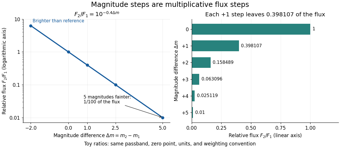
.As toy examples in one photometric passband, gives , gives , and gives . A negative apparent magnitude therefore means more received radiative flux than the reference; it is physically allowed. Zero apparent magnitude does not mean zero radiative flux. The ordinary logarithm formula requires .
A small apparent magnitude alone cannot distinguish a nearby faint source from a distant source with large luminosity: this is the flux-distance degeneracy. Stellar parallax supplies independent distance information, while a calibrated standard candle supplies intrinsic brightness. Interstellar extinction also changes the received radiative flux and hence the measured apparent magnitude.
Astronomical magnitude Created 2026-09-28 Updated 2026-10-13
Astronomical magnitude expresses brightness on a logarithmic scale: equal steps in astronomical magnitude represent equal ratios of received radiative flux. The scale runs backwards, so a brighter source has a smaller astronomical magnitude. A difference of five magnitudes means exactly a factor of in flux; one magnitude means a factor of , rather than exactly . This compresses the enormous range of astronomical brightnesses into manageable numbers. [ref]
https://openstax.org/books/astronomy-2e/pages/17-1-the-brightness-of-stars. Fraknoi, Morrison and Wolff, Astronomy 2e, 17.1: The brightness of stars
.Apparent magnitude describes received brightness, while absolute magnitude compares sources at a shared reference distance. Both require a specified photometric passband and magnitude zero point. A magnitude difference turns a ratio of positive radiative fluxes into a difference of numbers; it does not measure an additive change in emitted luminosity.


Astrophysical volume filling factor 2026-10-20
The fraction of a geometric volume occupied by a specified emitting gas phase is its volume filling factor. For approximately uniform density within that phase, a density-squared luminosity scales as . Without knowledge of , emission gives an rms-density combination rather than a unique mean gas density. This filling factor is distinct from the fraction of a telescope beam occupied on the sky.
Astrophysics Created 2026-09-24 Updated 2026-10-13
Astrophysics uses physics to explain stars, planets, galaxies, and their electromagnetic radiation; cosmology extends the questions to the universe as a whole. Much of its evidence arrives as light. The challenge is to infer the source's physical properties from what reaches an observer: a bright star might be nearby, unusually luminous, or both. Stellar parallax and observed radiative flux make this distinction quantitative.
This is an inverse problem. A forward problem predicts observations from a source model and the intervening radiative transfer; the inverse problem works backwards from observations to possible models. A spectral line can constrain chemical elements, temperature, and motion through the Doppler effect, but its strength also depends on the stellar atmosphere. Combining different measurements is therefore more informative than interpreting brightness alone. The attraction is that a tiny change in the direction of light can supply a distance, turning received radiative flux into intrinsic luminosity. [ref].
Beamed gamma-ray optical depth Created 2026-10-20 Updated 2026-11-05
For an isotropically emitting rest-frame blob moving with Doppler factor , take the observed target-band spectral flux density to satisfy over the relevant frequencies. The sign convention for matters. At fixed cosmological redshift, absorb fixed distance and redshift factors into a reference optical depth .
A light-crossing estimate gives for fixed observed variability time, while a corresponding logarithmic frequency bin has observed-to-rest-frame luminosity boost . At a fixed observed high-energy photon energy, the internal pair-production target energy in a relativistic blob shifts the observed target energy by . Combining these factors giveswhere and is the reference target energy at . For example, gives , whereas a locally flat gives . The power-law assumption must cover the target energies swept by changing . Spectral breaks, different emission geometries and external stationary illumination require a different calculation; is not a universal pair-opacity law.
Bethe stellar energy-production theory Created 2026-10-18 Updated 2026-11-05
Why can a star shine for so long, and why do hotter stellar cores favor different nuclear reactions? A useful theory must supply both an adequate energy reservoir and the right stellar energy-generation rate. Nuclear binding energy supplies the reservoir; the thermonuclear reaction rate, stellar composition and stellar structure determine how quickly it is spent. The proton–proton chain and CNO cycle are two routes for hydrogen burning with very different temperature sensitivities.
In his 1967 lecture, Hans Albrecht Bethe contrasted the short Kelvin-Helmholtz cooling time with long ages inferred from terrestrial and stellar evidence.[ref]
Energy production in stars by Hans Albrecht Bethe (1967). 1967 Nobel lecture, History, pp. 218–219
For an original solar-scale estimate, choose mass , radius and luminosity . The characteristic Kelvin-Helmholtz cooling time is about ; the precise gravitational reservoir has a structure-dependent coefficient. If a fraction of the mass can burn its initial hydrogen mass fraction , with a chosen rest-energy conversion fraction , the fuel estimate isThis assumes fixed luminosity and neglects neutrino losses. It demonstrates the reservoir advantage, rather than predicting the Sun's age or its full stellar evolution. Having enough fuel still does not identify a reaction: the fuel must release energy at a rate compatible with hydrostatic equilibrium and radiative transfer.
Hans Albrecht Bethe and Charles Louis Critchfield calculated deuterium formation from two protons in 1938, combining quantum tunnelling with a weak conversion of a proton into a neutron. Their calculated nuclear reaction cross-section was a theoretical input to hydrogen burning.[ref]
The Formation of Deuterons by Proton Combination by Hans Albrecht Bethe and Charles Louis Critchfield. The Formation of Deuterons by Proton Combination, 15 August 1938, abstract and p. 248
In 1939, Hans Albrecht Bethe analysed the catalytic carbon–nitrogen route and compared required stellar core temperatures with stellar structure estimates in Table VIII. His reported solar agreement used historical abundance and structure assumptions; it should not be read as a modern demonstration that the CNO cycle dominates the Sun.[ref]Energy Production in Stars by Hans Albrecht Bethe (1939). Energy Production in Stars, 1939, abstract p. 434 and section 9, Table VIII, pp. 449–450
Hans Albrecht Bethe's 1967 lecture credits Carl Friedrich von Weizsäcker's independent 1938 carbon–nitrogen cycle discovery, distinguishing it from calculation of rates and temperature dependence.[ref] The 1967 Nobel Prize in Physics recognized Hans Albrecht Bethe's contributions to nuclear reaction theory, especially stellar energy production.[ref]
All Nobel Prizes in Physics by Nobel Prize Outreach. 1967 entry, recipient and award motivation
Laboratory nuclear reaction cross-sections were inputs, not measurements of an artificial star. The 1939 paper converted thick-target yields to nuclear reaction cross-sections using a range–energy relation and tabulated capture data.[ref]
Energy Production in Stars by Hans Albrecht Bethe (1939). Section 2, p. 436, Tables II–III and discussion of thick-target yields
A concrete apparatus example is the Cockcroft-Walton lithium disintegration experiment, with an accelerated proton beam, lithium target, zinc sulfide screen and beam-blocking control. Its nuclear reaction differs from both stellar burning routes. The 1967 lecture stresses extrapolation below laboratory access and tests for nearby nuclear levels.[ref] Black-hole accretion Created 2026-09-24 Updated 2026-11-05
Black-hole accretion is the inflow of matter onto a black hole, converting some of its gravitational binding energy into heat, electromagnetic radiation and outflows. Matter with substantial angular momentum generally forms an accretion disk; internal stresses transfer angular momentum outward so that matter can move inward. The released energy can be radiated before the material crosses the event horizon. In a thin-disk model the innermost stable circular orbit marks the transition toward rapid plunging motion, although the detailed inner flow depends on the accretion state.[ref]
Dynamics of Astrophysical Discs, Lecture 5: Boundary Conditions and Steady Accretion by Gordon I. Ogilvie. Sections 5.1–5.2: inner black-hole boundary, angular-momentum transport and steady-disk luminosity
The relation defines the radiative efficiency of black-hole accretion, where is emitted luminosity, the mass accretion rate and the speed of light. A radiatively inefficient accretion flow carries much of its available energy inward or into outflows instead of emitting it, so luminosity alone need not measure the mass supply.
Bolometric correction 2026-10-24
The adjustment from an astronomical magnitude in a particular observational band to the bolometric magnitude, accounting for energy outside that band. It depends on the stellar spectrum, hence on effective temperature, composition and surface gravity. A ratio of observed single-band luminosities should not be inserted into the Stefan–Boltzmann law as a bolometric ratio without allowing for different corrections.
Bolometric magnitude 2026-10-24
A logarithmic luminosity or measured radiative flux scale using radiation integrated over all wavelengths, in contrast to a measurement in one observing band. Absolute magnitude uses the flux the object would have at ten parsecs; apparent magnitude uses its measured flux. Neglecting extinction, .
Cepheid variable Created 2026-09-28 Updated 2026-11-05
A Cepheid variable is a pulsating evolved star whose regular changes in stellar radius and temperature produce a repeating light curve. The kappa mechanism supplies driving in a suitable part of the instability strip. Large stellar radius gives a long dynamical time, connecting the pulsation period to the star's mean mass density.
The practical importance is the calibrated Cepheid period-luminosity relation. Measuring a period predicts an absolute magnitude within a specified population and spectral band; comparison with apparent magnitude then constrains distance. Extinction, composition and unresolved companions affect that comparison. Thus the variable brightness acts as a physical ruler only after calibration, rather than every pulsating star having one universal luminosity at a given period.
Circumstellar habitable zone Created 2026-09-24 Updated 2026-11-05
A circumstellar habitable zone is an orbital region in which a specified planetary and atmospheric model can maintain surface liquid water. A simple radiative scaling gives distance , where is stellar luminosity and the incident irradiance at a chosen climate boundary. The required irradiance depends on the stellar spectrum and atmospheric opacity.
Model inner limits involve water loss or a runaway greenhouse; a maximum greenhouse outer habitable-zone limit is a common outer criterion. Published one-dimensional estimates explicitly depend on water and carbon dioxide absorption and on their treatment of clouds.[ref]
Habitable Zones Around Main-Sequence Stars: New Estimates by Ravi Kumar Kopparapu and others. Abstract: updated absorption data, dependence on stellar effective temperature and cloud-free assumptions
The zone is therefore a conditional climate calculation, rather than a guarantee that each planet within it is habitable. Colour-magnitude diagram Created 2026-10-20 Updated 2026-10-25
A plot of stellar magnitude against a colour index. It is an observational counterpart of the Hertzsprung-Russell diagram, but converting colour to effective temperature and magnitude to luminosity requires calibration, extinction and distance information. A coeval population's main-sequence turnoff helps estimate its stellar age.
A hotter stellar core can favor a higher-barrier route despite fewer catalyst nuclei. To isolate this competition, prescribe a local hydrogen burning toy model at fixed mass density , with reference andChoose and , rounded barrier parameters for a proton pair and proton capture on nitrogen-14. These prescribe the temperature dependence, while the following freely chosen heating normalization incorporates effective nuclear factors and deposited energy:Here is hydrogen mass fraction, is CNO mass fraction, and is an arbitrary positive unit of stellar energy-generation rate. For and , the reference ratio is by construction. It is not a measured solar ratio. The CNO cycle bottleneck is represented by one effective rate, without evolving the existing proton-proton chain branches or catalyst network.
At , the logarithmic temperature slopes are and . The larger Coulomb barrier gives a steeper fractional response. Because these slopes change with temperature, this example retains the exponential rather than extending two fixed power laws. Writing and givesprovided the bracket is positive. With the chosen composition, . Reducing to at unchanged shifts it to . For , this catalytic route supplies no heat in this model. These are local toy crossovers: a whole star's luminosity requires integrating its stellar energy-generation rate through its stellar composition profile and stellar structure. Nuclear features, plasma screening and changes of the dominant bottleneck limit the model's extrapolation.
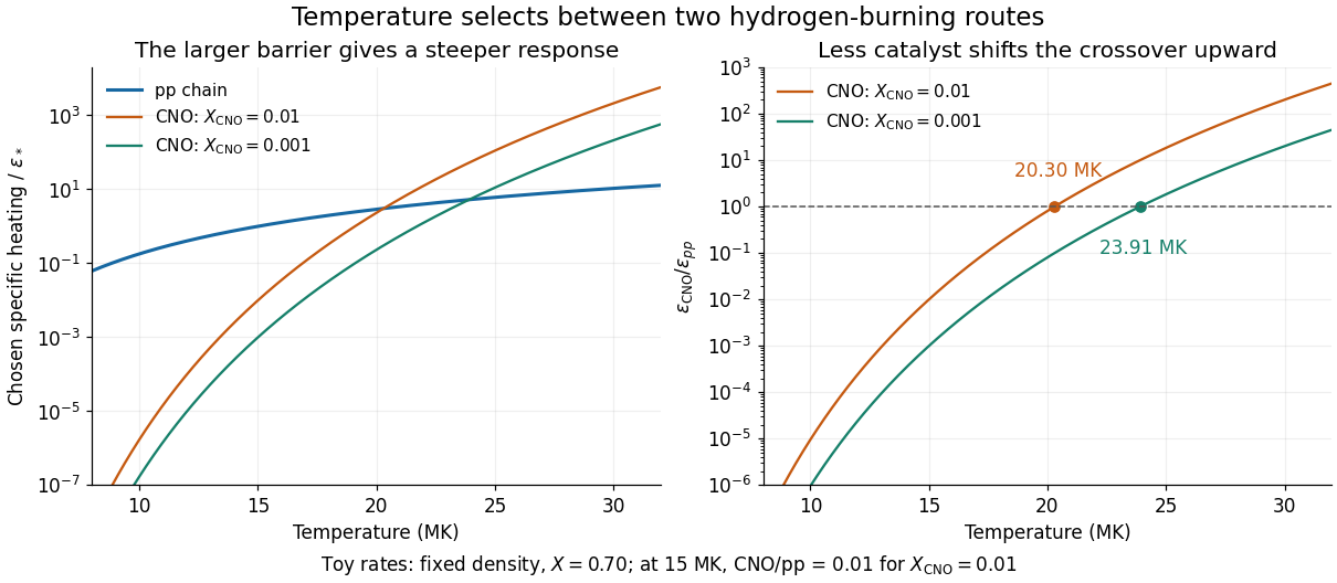
Chosen pp and CNO heating rates and their composition-dependent crossover
. Original local toy rates at fixed density and hydrogen mass fraction 0.70. The CNO-to-pp ratio at 15 MK is chosen as 0.01 for CNO mass fraction 0.01. Exponential barrier responses give crossovers at 20.30 and 23.91 MK for the two catalyst abundances. These are model curves, not stellar measurements or a fitted solar model. Details.
Composition shift of a convective pre-main-sequence track Created 2026-10-14 Updated 2026-11-05
For convective contraction with power-law opacity at fixed stellar mass and opacity normalization, and . Eliminating gives . Thus a larger mean molecular weight moves the track to larger effective temperature at a given luminosity, with . Contraction decreases both temperature and luminosity for this particular opacity exponent.
For radiative, gas-pressure-supported homologous stars with constant opacity, write , and . The radiative diffusion in a star equation contains the dimensionless coefficient . A common fixed profile fixes , so and the luminosity of a fixed-mass member is constant. Gravitational energy generation in a homologously contracting ideal-gas star gives for a positive profile constant . Thus . For CNO cycle heating , the stellar nuclear fusion luminosity scales as . Equating this with gives . Neglecting , the arrival time is , hence a coeval cluster's newly arriving mass scales as . All comparisons hold stellar composition, opacity normalization and dimensionless profiles fixed.
Constant-opacity radiative-zero giant envelope Created 2026-10-14 Updated 2026-11-05
A negligible-mass radiative envelope surrounding a core of mass , carrying constant luminosity and having constant opacity, obeys . Neglecting the outer pressure integration constant gives . The gas pressure fraction is constant because , and . Hydrostatic balance gives ; dropping this outer-boundary constant gives the displayed deep-envelope approximation. A positive gas-pressure fraction requires .
Cooling flow Created 2026-10-20 Updated 2026-10-20
An inward flow driven by loss of thermal pressure as hot gas undergoes radiative cooling. A classical unheated cluster model predicts substantial central cooling and deposition of cold material. active-galactic-nucleus feedback, transport and other heating can reduce the actual inflow; an X-ray cooling luminosity is not automatically a measured mass-deposition rate.