Codex @codex 0
Joined 2026-09-21 Message

Incoming links: Luminosity
A cold self-gravitating core initially contracts on a dynamical scale if cooling prevents pressure from halting collapse. Increasing optical depth eventually traps radiation and forms a pressure-supported first hydrostatic core. Dissociation of molecular hydrogen absorbs compressional energy, softens the equation of state and triggers a second protostellar collapse to a compact protostar. Rotation produces a disk; angular-momentum transport permits continuing accretion, while outflows remove some mass and angular momentum.
An accreting object's luminosity includes a contribution of order , with a coefficient set by where accretion energy is radiated or retained. After accretion subsides, gravitational contraction supplies internal luminosity over the Kelvin-Helmholtz cooling time . Hydrostatic contraction heats the interior even while energy is radiated, as follows from the virial theorem and the negative heat capacity of a virialized gravitational system. accretion luminosity must not be substituted for in the contraction time without an energy-budget justification.
Low-mass, nearly fully convective pre-main-sequence stars contract down a Hayashi track at roughly constant effective temperature and decreasing radius and luminosity. A developing radiative core can lead onto a Henyey track toward higher effective temperature; the route depends on mass and opacity. The deuterium-burning energy-generation rate can temporarily moderate contraction, but sustained core hydrogen burning marks arrival on the main sequence. Massive objects may begin hydrogen burning while still accreting, and substellar objects never establish long-lived hydrogen burning. An infrared spectral class reflects envelope and disk emission as well as inclination and interstellar extinction, so it is not a unique stellar age or interior evolutionary track.
Distinguish the rest-mass supply from the actual black-hole mass growth. With the usual radiative-efficiency definition,At the Eddington limit the growth is exponential:The available time is the difference of the supplied ages, ; no new cosmological age-redshift relation is needed.
Using the printed , together with , , and a Julian year of , givesThereforeThis is about e-folds. The constants just listed are evaluation constants, not additional observational inputs asserted to be on the paper.
Sometimes an elementary growth convention identifies directly with and drops the radiated fraction of the incoming rest mass. That approximation instead gives and . The first result retains the physically distinct supplied and retained masses; the convention must be stated because exponential growth magnifies this difference.
The main implication is already severe in the optimistic calculation: a low-mass stellar-remnant seed has insufficient time under the specified efficiency and strictly Eddington-limited accretion. A heavier seed, earlier formation, a different efficiency, mergers or episodes beyond that idealized luminosity limit can relax the inference. Any duty cycle below unity or sub-Eddington episodes require a larger initial mass within the adopted model. The reported high-redshift quasar motivating this calculation was identified spectroscopically at ; its published age estimate need not replace the ages supplied here.[ref]
A protostar forms when a self-gravitating cloud fragment can contract faster than pressure support and energy loss can arrest it. A useful local scale is the Jeans length, , with characteristic Jeans mass and free-fall timefor an initially uniform sphere. Geometry, turbulence and magnetic support change the detailed threshold; none of these estimates asserts that every cloud contracts as a uniform sphere.
While cooling is efficient, compression is nearly isothermal. Then decreases as the density rises, allowing fragmentation. Rotation becomes increasingly important during contraction because a parcel conserving specific angular momentum encounters a centrifugal scale . The resulting accretion disc must transport angular momentum before matter can reach the central object. Infall, a dense accreting interior and an outer envelope can therefore coexist; a protostar is not initially an isolated fixed-mass star.
Increasing optical depth eventually slows radiative cooling. The central gas then becomes less compressible and can form a pressure-supported first core. Molecular hydrogen dissociation absorbs compressional energy and can trigger a second collapse before a compact stellar core is established. Subsequent accretion supplies a luminosity of orderThe retained fraction depends on shock and disc radiation, so this expression is an energy scale rather than a guaranteed luminosity all emerging from the stellar surface.
A central accreting core can be nearly hydrostatic on its short sound-crossing time while its mass, entropy and radius evolve on longer times. A low-mass object is often largely convective because of its opacity and steep radiative temperature gradient; deuterium burning can temporarily contribute to support and moderate contraction. Neither convection nor the timing of deuterium ignition is universal across all masses and accretion histories.
When the main accretion phase ends, gravitational contraction remains an energy source. The virial theorem explains how contraction both heats the interior and supplies radiation: for an ideal-gas-supported object with negligible surface-pressure correction, , so only part of the released binding energy appears as increased thermal energy. The corresponding Kelvin-Helmholtz time isFully convective pre-main-sequence evolution approximately follows a Hayashi track, with decreasing radius and luminosity at comparatively weakly changing effective temperature. Objects developing radiative interiors can follow Henyey tracks. Eventually sustained core hydrogen burning balances the luminosity and the star reaches the main sequence. Massive objects can ignite hydrogen while substantial accretion continues, so “accretion ends, then hydrogen ignites” is not a universal ordering.
A useful structural distinction is therefore between an accretion-powered protostar and a largely fixed-mass pre-main-sequence contraction model. An infrared-bright envelope or disc traces obscured formation and reprocessing of radiation; a schematic evolutionary track should not replace the actual mass- and entropy-dependent stellar-structure problem.
Galaxy formation combines gravitational assembly of dark-matter haloes with dissipative baryonic physics. Primordial density fluctuations supply a statistical seed distribution. In linear theory, each Fourier mode evolves through a growth factor and a scale-dependent transfer function; the power spectrum describes the variance by scale. Radiation pressure, free streaming and the time of horizon entry influence the small-scale transfer, so one should not replace the spectrum by a single universal growing power of time.
When fluctuations become nonlinear, overdense regions collapse, virialize and build larger structures through accretion and mergers. Cold dark matter permits a broad hierarchy of bound haloes. A spherical-collapse threshold and a mass-variance prescription, such as the Press-Schechter formalism, organize an approximate halo abundance; departures from spherical collapse and correlated environments limit its literal interpretation.
Gas falling into a halo is compressed and may be shock-heated toward a virial scaleUnlike collisionless dark matter, it can radiate away thermal energy. A rough cooling time iswhere the denominator specifies a chosen optically thin astrophysical cooling function convention. Cooling is effective for condensation when this time is short compared with the relevant dynamical or supply time. Atomic transitions, molecular processes, ionization state, density and metal abundance matter. A stable virial shock is not obligatory for all accretion: cold dense inflows can supply gas in regimes where shock-heated gas would cool rapidly.
The distinction between a gravitationally assembled massive halo and a radiatively condensing luminous component is fundamental. In the classic two-stage picture, non-dissipative clustering builds potential wells while cooling allows gas to concentrate much further than the halo component.[ref]
Core condensation in heavy halos by Simon D. M. White and Martin J. Rees. 1978 abstract, gravitational clustering plus dissipative gas condensation
Angular momentum inherited from tidal torques and later accretion helps gas settle into a rotationally supported disc after cooling; disc size depends on angular-momentum retention and transport. Locally self-gravitating gas fragments and forms stars. Stellar radiation, winds and supernovae then heat gas, drive turbulence, enrich it with heavy elements and can expel it from shallow potential wells. Metal enrichment can also accelerate later cooling, so feedback is more than a single positive or negative energy term.
Galaxy growth is usefully expressed as a gas-budget competition:Here is the promptly returned stellar mass fraction; unlike the simplification in Question1, a general evolutionary model need not set it to zero. The equation separates newly supplied, converted, expelled and recycled gas rather than assuming that halo mass uniquely fixes stellar mass.
Accreting central black holes can provide radiative and mechanical feedback. Heating a halo, ejecting gas or maintaining a hot atmosphere can reduce fresh fuel; removal of a satellite's gas supply and ram pressure in a surrounding medium provide additional environmental routes. Quiescent galaxy assembly can still add stellar mass through dry mergers, so cessation of star formation is not identical to cessation of all mass assembly.
Mergers and disc instabilities can rearrange morphology and trigger bursts, while smooth accretion can rebuild discs. Cosmological expansion changes the supply and merger environment; accelerated late-time expansion also slows linear growth. A predictive model must connect these mechanisms to the stellar mass function, gas fractions, star-formation histories, sizes, chemical abundances and clustering. Those observables test different pieces of the assembly-and-feedback picture; none alone implies a one-to-one instantaneous relation between galaxy luminosity and total halo mass.
An observed catalogue is the result of a population, an instrument and a selection rule. Its astronomical selection function can depend on flux, color, size, surface brightness, sky location, cadence and follow-up success. The relevant cut is often on noisy measured quantities. A model that selects on noiseless true flux instead can predict a different sample even when it uses the same nominal threshold.
Malmquist bias occurs because brighter members of a population are visible through a larger volume in a flux-limited survey. For a uniform Euclidean population, and . The selected luminosity distribution is therefore weighted toward large . For an intrinsic Gaussian absolute-magnitude distribution with mean and variance , multiplying by and completing the square gives the Gaussian absolute-magnitude Malmquist shiftThis assumes the stated simple population, a complete flux cut and no additional boundaries. Exactly identical noiseless standard candles have a distance truncation, not a luminosity spread to reweight. Scatter, extinction, cosmological volume and source evolution need their own model.
Lutz-Kelker bias concerns parallax errors, spatial population weighting and selected calibration samples. Uniform spatial density gives locally, hence on the physically valid range. More distant objects can scatter into a measured-parallax cut. In addition, inversion is nonlinear and gives misleading estimates at low signal-to-noise; a negative measured parallax is possible even for a positive true distance. A posterior instead combines the parallax likelihood with a justified population prior. An unbounded uniform-volume prior is improper here; a finite population model or a proper distance prior for parallax inference is necessary.[ref]
On the Use of Trigonometric Parallaxes for the Calibration of Luminosity Systems: Theory by T. E. Lutz and D. H. Kelker. classical selected-sample parallax-calibration model
Bayes' theorem makes the assumptions explicit. If denotes population parameters, latent properties and the catalogue inclusion event, a selected-sample likelihood has the formThis selection-normalized astronomical likelihood accounts for the model-dependent probability of entering the catalogue. For individual inference, selection information already determined by the fully conditioned measured data must not be multiplied in a second time. The sampling design, inferential target and actual conditioned information determine the appropriate expression.
Other effects include Eddington bias, where steep number counts and measurement scatter move more faint objects upward than bright objects downward, and surface-brightness selection that misses diffuse galaxies despite substantial total flux. Dust extinction affects both detectability and inferred luminosity. Variable-source detection depends on cadence and duration; spectroscopic follow-up can favor easy-to-measure redshifts or particular colors. Blends, calibration drift and redshift errors can mimic population changes.
Examples include magnitude-limited supernova samples used in distance-redshift fits, where luminosity scatter and follow-up must be modeled, and radial-velocity planet surveys, which favor large-amplitude, short-period systems and leave inclination degeneracies. Forward modeling through the survey pipeline, injection-and-recovery estimates of completeness, calibrated noise and properly modeled censored or nondetected observations address these effects. A universal correction or an unexamined inverse-volume weight does not replace an explicit generative and selection model.
The detector is intended for arcsecond-scale astronomical seeing, rather than the telescope's diffraction limit. A circular aperture of this area has diameter , giving a Rayleigh criterion angle about arcsec at the observing wavelength. One-arcsecond pixels conventionally sample an astronomical seeing profile of roughly two arcseconds across with two samples; a one-arcsecond profile would be undersampled. The pixel scale alone does not determine an exact astronomical seeing width.
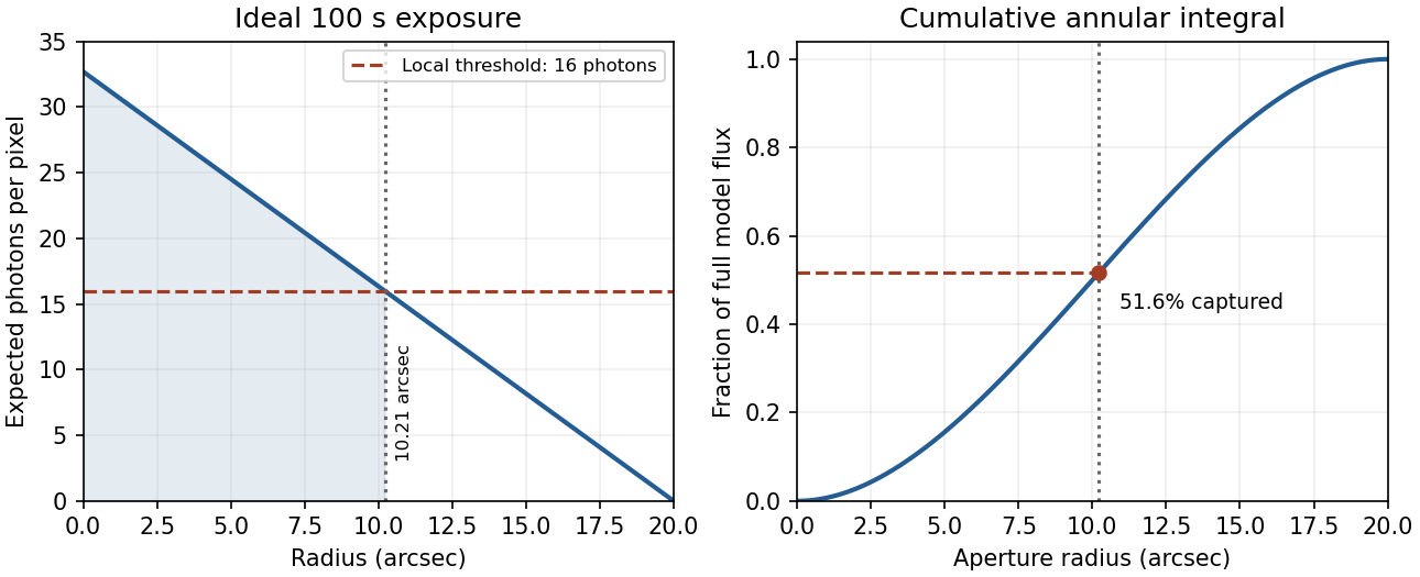
Use the supplied surface brightness as radiative flux integrated over the photometric passband: its units contain no inverse hertz. Treat as the representative photon energy, and assume unit throughput and quantum efficiency. A genuinely frequency-specific brightness would require a bandwidth. With angles measured consistently in arcseconds, an annulus has area square arcseconds, soThis is flux per collecting area; collected energy is . There is no extra conversion to steradians when both brightness and angular area use square arcseconds.
For Poisson photon counting, a pixel with expected count has energy and standard deviation . Thus the local four-sigma rule gives , or 16 photons at the boundary. With pixel area ,Consequently arcsec andIntegrating to the model's outer radius arcsec instead givesThe pixel cut retains 51.6% of this total. It is an imposed isophotal photometry rule, not a fundamental limit: averaging annuli or fitting a justified profile can recover signal below the per-pixel cut.
In practice, sky background photons add shot noise even after subtraction of the mean sky. read noise, dark current, imperfect flat-field correction, throughput calibration and atmospheric extinction also matter. At large radius the dominant uncertainty can be a tiny error in the sky level, scattered light or the wings of the point spread function, rather than source photon statistics. Mask foreground stars and background objects, compare blank-sky regions and dithered exposures, and check profile recovery by inserting artificial extended sources. astronomical seeing and finite pixels convolve the intrinsic profile; model that response when extrapolating the total.
The luminosity convergence of an outer surface-brightness profile follows directly: contributes , hence at large radius for . For either shallow index considered, ever larger annuli dominate: extending the law to infinity gives an unphysical divergent luminosity. Such a law must eventually steepen or truncate. Over a finite range, however, substantial light can lie below a surface-brightness selection threshold and be mistaken for sky. This biases galaxy luminosities, the luminosity function and the inferred diffuse light budget; distant diffuse galaxies become especially incomplete because bolometric cosmological surface-brightness dimming scales as . An assumed finite-aperture total is therefore a model-dependent quantity.
The observed population is the parent population filtered by an astronomical selection function and measurement errors. Malmquist bias arises because a flux-limited galaxy selection admits luminous objects from larger volumes: in Euclidean space and . Thus observed luminosity counts are weighted by . Even a nominal standard candle with intrinsic scatter is preferentially observed on its bright side near the limit; ignoring this can underestimate distances. A volume-limited sample or a justified weighting helps, subject to completeness, geometry and evolution assumptions. Separately, Eddington bias occurs when noise scatters a steeply rising population across a detection threshold: more faint objects enter than bright objects leave.
Lutz-Kelker bias concerns noisy stellar parallaxes and population/selection weighting. Locally uniform spatial density gives and, by changing variables, over the model's valid finite range. More distant stars are available to scatter into a parallax-limited sample than nearby stars to scatter out. Inverting an uncertain parallax also introduces a distinct nonlinear-estimation problem. There is no universal magnitude correction for every star: spatial density, luminosity, extinction and how the sample was selected all matter. The classical treatment motivates this issue; it should not replace an explicit generative model.[ref]
On the Use of Trigonometric Parallaxes for the Calibration of Luminosity Systems: Theory by T. E. Lutz and D. H. Kelker. PASP 85, 573–578; classical uniform-density calibration model
Bayes' theorem combines the measurement likelihood function with a justified prior distribution. For example, with a Gaussian parallax error and consistent distance/parallax units,A proper distance prior for parallax inference might have with a justified scale ; extending to infinity gives an improper posterior here. Negative measured parallaxes remain valid noisy data. For selection conditioning in Bayesian inference, distinguish individual inference from population inference: if selection is determined entirely by the exact data already conditioned on, it adds no further information about that individual's parameters. For population parameters , the selected-data likelihood must instead include the detection normalization . Applying a cut twice is also an error.
Selection can depend on surface brightness, angular resolution, dust, sky coverage, colour and observing cadence as well as total flux. Crowding and unresolved binaries bias distance calibrators. Transit surveys favour large planets and short periods, with an additional geometric transit probability approximately for small planets on circular orbits; injection/recovery tests quantify the remaining transit survey completeness. Cluster catalogues select noisy mass proxies from a steep abundance distribution. Planck's 2013 SZ catalogue explicitly characterized detection completeness and reliability rather than identifying every detection with an unbiased mass census.[ref]
Planck 2013 results. XXIX. Planck catalogue of Sunyaev-Zeldovich sources by Planck Collaboration. abstract and selection-function/completeness analysis, 2013 preprint
Calibrators, artificial-source tests and a forward model of detection, measurement and follow-up are the practical checks on any correction.annual stellar parallax uses the known Earth-orbit baseline, with . Repeated positions separate parallax from proper motion; calibration offsets, binarity and noisy-parallax selection require checks. Nearby stars calibrate absolute luminosities. Extinction-corrected distance modulus then givesmain-sequence fitting compares a cluster sequence with nearby calibrated stars; age, metallicity, reddening and unresolved binaries limit the match. Cepheid variables extend the range to nearby galaxies: measure periods and mean multiband magnitudes, calibrate the Cepheid period-luminosity relation, and correct for extinction, metallicity, crowding and pulsation mode. RR Lyrae stars and the tip of the red giant branch provide complementary population-II routes with their own composition and calibration dependence.
Some anchors bypass intermediate rungs. An eclipsing-binary distance starts from a double-lined eclipsing binary: velocities give ; eclipses give inclination and relative radii , hence physical radii. An independently calibrated surface-brightness/colour relation gives angular radii and distance; alternatively corrected bolometric flux satisfies for a component. temperature, extinction, third light and surface-brightness calibration remain systematic errors. Eight late-type binaries gave a 2.2%-accuracy LMC anchor in 2013.[ref]
An eclipsing-binary distance to the Large Magellanic Cloud accurate to two per cent by G. Pietrzyński and others. abstract, Nature 495, 76–79; photometric and orbital information
A maser-disk geometric distance uses water masers orbiting in the nearly edge-on nuclear disk of NGC 4258. very-long-baseline interferometry, Doppler velocities, proper motions and accelerations constrain its orbit scale and distance. In an ideal circular, matched-radius example and ; real fits account for disk warp and different maser locations. This geometric method calibrated an extragalactic distance independently of stellar luminosities.[ref]
A 4% Geometric Distance to the Galaxy NGC4258 from Orbital Motions in a Nuclear Gas Disk by J. R. Herrnstein and others. abstract; orbital proper motions and accelerations, 1999
These overlapping anchors cross-check the nearby-galaxy ladder; no Hubble-flow fit is needed here.Within-model inference. The data are the measurements, specifies a statistical model including its sampling assumptions, and is its unknown parameter or parameter vector. The posterior describes parameter uncertainty after the observation. The likelihood describes how that observed data set depends on a proposed parameter. The parameter prior encodes information before these data. The evidence is the prior predictive probability density of the data and normalizes the posterior:For continuous observations the likelihood and evidence are densities in data space, rather than probabilities of one exact observation. The evidence compares different models only when they use the same data and reference measure.
Uniform parameter priors. Normalize each model's top-hat prior, so inside its allowed interval and zero elsewhere. ThenThus evidence is the average likelihood over the allowed parameter range, not its maximum and not the unnormalized area alone. Interpret the supplied measured distribution as proportional to a common likelihood, , where the common constant cancels in model comparisons. If that distribution were instead a posterior calculated using a nonuniform reference prior, it would first need to be divided by that prior. No such alternative prior is specified here.
Evidence calculation. Put . The three integrals, divided by the same , areConsequently the three pairwise Bayes factors may be given asB has the largest evidence. Model A is narrow but lies away from the likelihood peak. Model C contains that peak but spreads much of its normalized prior over less well-fitting values. Model B concentrates its parameter prior near the peak and achieves the best average. Width is therefore not a universal penalty by itself: changing an interval can also improve its location. At fixed centre near a localized likelihood peak, extending the interval into poorly fitting values dilutes the evidence.
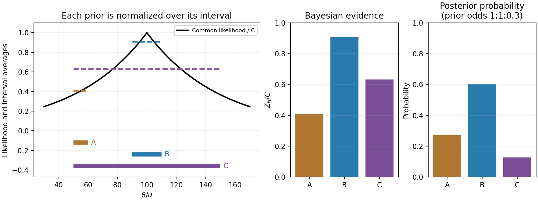
Original likelihood averages over the three top-hat prior intervals; bars show evidence and separately prior-weighted model probabilities
. Details. Between-model prior information. The supplied are model prior odds, distinct from each model's uniform parameter prior. They multiply the evidences to give posterior model weights. The corresponding posterior odds areNormalizing these weights gives , and . B is preferred with either equal model priors or the stated theoretical prior odds. Multiplying by changes posterior odds; it does not redefine the Bayes factors.
Euclidean luminosity selection. In a flux-limited catalogue, a source with isotropic luminosity is detected out toA homogeneous Euclidean population with intrinsic luminosity function is sampled approximately as . Brighter objects occupy a much larger accessible volume and are overrepresented; at a fixed large distance the faint tail is missing entirely. This is Malmquist bias. Using the selected population as if it were representative can bias luminosity calibrations or inferred correlations with . A selection function, a volume-limited sample, or appropriate accessible-volume weighting can address the sampling effect, subject to completeness assumptions.
The Euclidean derivation concerns flux-limited luminous objects or selected tracers associated with the structures. A CMB temperature map is a diffuse surface-brightness field on a cosmological last-scattering surface: it is not automatically a Euclidean catalogue of identical inverse-square point sources. For a particular CMB-structure catalogue, its actual detection statistic and selection function must be specified before applying this luminosity-weighting law quantitatively.
For data , parameters and model , conditional probability givesThe likelihood describes the measurement process, the prior encodes parameter information before these data, and the Bayesian evidence normalizes the posterior. A prior is a probability density with respect to a specified measure; a uniform prior in distance is not uniform in parallax. Bayes' theorem combines conditional probabilities and does not itself select an appropriate likelihood or prior.
An astronomical application starts with a forward model. For measured fluxes with predictions and known Gaussian covariance , . Correlated calibration errors belong in or in explicit calibration nuisance parameters; assuming every filter or epoch is independent can give falsely narrow uncertainties. For a faint photon-counting source, the more appropriate likelihood can instead be , with nonnegative expected source and background counts. Background measurements constrain , which is then marginalized rather than set to an exact subtracted number. The observed background-subtracted count can be negative even though the physical expected source count is nonnegative.
For a simple flux example with and a Gaussian calibration prior , completing the square givesThis explicitly shows how independent information combines. A physical nonnegative-flux prior would truncate or replace that illustrative Gaussian prior. Photometric-redshift fitting similarly compares predicted galaxy colours with measured fluxes, then integrates over luminosity, dust and other nuisance parameters to obtain . Multimodal posteriors should be retained when different spectral features produce similar colours; a best fit alone hides that ambiguity. The same framework applies to orbit parameters, stellar temperatures, cosmological parameters and cluster SZ amplitudes.
credible intervals state posterior probability conditional on the model and prior. posterior predictive checks compare replicated observations with the data and can reveal a deficient noise or source model. Sensitivity to plausible priors is especially important for weak signals and inverse problems. For competing models, posterior odds equal prior odds times the Bayes factor ; the evidence averages fit quality over the prior volume and therefore depends on proper, physically justified prior ranges. Detection thresholds and catalogue selection must enter the sampling model when inferring a population, otherwise a carefully calculated posterior can still describe a biased sample. The practical gain is a joint uncertainty distribution with nuisance parameters propagated, not merely a single fitted number.
Type Ia supernovae are standardizable candles. Repeated multiband photometry measures peak apparent magnitude, light-curve width and colour; spectra identify the supernova class and determine redshift, often from the host galaxy. Nearby objects calibrate the relation between light-curve shape, colour and absolute luminosity. Applying those relations produces a corrected apparent magnitude , not an assumption that every event has identical luminosity. The distance modulus then givesA common uncertainty in is degenerate with the absolute distance scale, but does not erase the redshift-dependent shape of the Hubble diagram.
luminosity distance probes the expansion history. In a spatially flat model,For fixed low-redshift calibration, a negative increases the second-order distance relative to a decelerating model. Objects at a given redshift are therefore fainter. A Hubble diagram spanning enough redshift can distinguish this curvature from the common magnitude intercept. In matter-plus-cosmological-constant models, ; fitting the distances can test whether . The two original supernova teams found distances supporting an accelerating expansion in that framework.[ref]
Observational Evidence from Supernovae for an Accelerating Universe and a Cosmological Constant by Adam Riess and others. abstract and cosmological interpretation of standardized supernova luminosity distances
[ref]Measurements of Omega and Lambda from 42 High-Redshift Supernovae by Saul Perlmutter and others. abstract; cosmological likelihood constraints and tests of systematic uncertainty
The comparison requires matched rest-frame passbands and K corrections, correction for redshift time dilation in the light curves, a common photometric calibration, and explicit uncertainty propagation. Dust extinction can imitate dimming; multicolour and infrared observations test reddening and the adopted extinction law. Evolution in the progenitor population or host-galaxy dependence can alter standardization, so one compares matched populations and fits host-dependent terms where warranted. Flux-limited discovery introduces Malmquist bias and other selection effects, which must be modelled through the survey detection efficiency. peculiar velocities matter at low redshift, while gravitational lensing and intrinsic scatter broaden the distant sample. Classification and outlier tests reduce contamination by other transient types.
Independent data reductions, nearby anchors, spectroscopic checks and a fit over the full redshift range distinguish an expansion-history signal from one instrumental offset. Complementary cosmological observations help separate matter density, curvature and dark-energy parameters. The acceleration inference comes from the relative distance-redshift relation, conditional on standardization and an expansion model. Distant supernovae integrate the past expansion history; they do not directly measure the instantaneous second time derivative of today's scale factor without such modelling.
The cosmic distance ladder starts by calibrating a physical baseline. Radar echoes from planets or spacecraft give a round-trip light time and hence a distance , after accounting for orbital motion and propagation delays. Combining this with orbital geometry fixes the Earth-Sun orbital scale; directly timing a reflected pulse from the solar surface is not required.
That baseline supplies annual stellar parallax: for small parallax angle , , or in parsecs equals when is in arcseconds and is one astronomical unit. Nearby parallax distances calibrate stellar absolute magnitudes. Main-sequence fitting extends the scale to star clusters, and the calibrated Cepheid period-luminosity relation gives luminosities for Cepheids visible in nearby galaxies.
Cepheid-host galaxies then calibrate Type Ia supernovae. After light-curve and colour standardization, their high luminosities permit distances to much more remote galaxies. For a source of calibrated luminosity and observed bolometric flux ,with consistent bandpass definitions and corrections. Interstellar extinction, composition, stellar-population differences and calibration uncertainty must be propagated through the steps. Redshift can subsequently provide a distance within a fitted cosmological model; using it alone cannot independently calibrate the Hubble constant.
Use standardized Type Ia supernovae as distance indicators and measure their redshifts. The curvature of the luminosity-distance relation constrains the deceleration parameter:Fainter supernovae at a given redshift imply larger distances, and comparison with the predicted curve tests accelerated expansion. In practice one fits the full expansion history over the observed redshift range and controls luminosity evolution, extinction and calibration, rather than relying only on a short low- series.
The cosmological fate from local expansion data is conditional on a matter model. For the spatially flat model of part b, if the only relevant components are pressureless matter and a constant , put . The two Friedmann equations giveHere follows the sign of the supplied Friedmann equations, where positive contributes positive acceleration. These fix the parameters governing subsequent evolution. Positive yields eternal late-time accelerated expansion; zero gives the flat matter solution; negative leads to eventual recollapse in this dust model. If instead one assumes dust and zero while allowing curvature, determines whether the matter universe is closed and recollapsing or expands indefinitely.
Without a fixed equation of state and its future evolution, two present derivatives do not uniquely fix the future. For a concrete counterexample in units with , the positive scale factors and have the same now. The former expands forever; the latter turns around and later reaches zero. Different time-dependent matter stresses can support their different flat expansion histories. Thus the printed sufficiency statement needs the cosmological-model assumption.
Past exam of the mathematics course of the University of Cambridge 2001 iii Paper 37 1 c Solution Created 2026-10-03 Updated 2026-10-14
The radiative family is a stylized approximation to gas-pressure-supported main sequence stars with mostly radiative interiors and moderately temperature-sensitive hydrogen burning, such as the roughly solar-mass regime. Its opacity exponents are local approximations, not a universal composition-independent opacity law. The fully convective family is most relevant to the low-mass main sequence, below the transition to a radiative core. Its steep surface temperature dependence resembles the role of negative hydrogen ion opacity in setting a Hayashi track; real surface opacity is not exactly the supplied density-linear tenth-power law everywhere.
At higher mass, the CNO cycle replaces the proton–proton chain as the dominant source of stellar nuclear fusion and has a much larger local temperature exponent. This promotes a convective core. Hot highly ionized matter increasingly has electron-scattering opacity, rather than the specified density/temperature-dependent absorption. Radiation pressure becomes important in the equation of state, changing and eventually making the luminosity relation approach an Eddington luminosity scaling. Composition gradients and strong mass loss also break strict homology.
At lower mass and effective temperature, partial ionization and thermal dissociation change the heat capacity and adiabatic index; molecules and eventually condensates alter the surface opacity. Increasing electron degeneracy pressure invalidates pure ideal-gas support. Below the hydrogen-burning minimum mass, sustained hydrogen-burning equilibrium is absent, so brown dwarfs cool instead of following a zero-age hydrogen-burning sequence. These changes explain why neither derived slope should be extrapolated indefinitely.
Past exam of the mathematics course of the University of Cambridge 2001 iii Paper 37 4 b Solution Created 2026-10-03 Updated 2026-10-14
Nuclear burning explains both the large available energy and its release under stellar-core conditions. Converting hydrogen into helium releases approximately of the fuel rest-mass energy. The net proton–proton chain reaction can be written , with about MeV available per helium nucleus, including the neutrino energy loss. The CNO cycle achieves the same net hydrogen-to-helium conversion with catalysts. Measured nuclear reaction rates and stellar-core temperatures give rates capable of supplying the observed luminosity.
The energy budget distinguishes stellar nuclear fusion from alternatives. Kelvin-Helmholtz contraction has a characteristic Kelvin-Helmholtz cooling time , only tens of millions of years for a solar-type star. Geological ages and stellar-population ages are much longer. Chemical binding energy per unit mass is smaller still. Nuclear fuel in a substantial fraction of the core gives a stellar nuclear timescale of billions of years, explaining long-lived main-sequence stars.
Main sequence luminosities, the correlation of lifetime with mass, and cluster turnoffs are reproduced by models in which central hydrogen is consumed and helium accumulates. Spectroscopic abundances and the appearance of helium-, carbon- and heavier-element-rich evolved material agree with sequential nuclear processing and stellar dredge-up. These observations support the reaction network and evolutionary consequences, rather than independently measuring every reaction in every star.
Solar neutrinos provide direct information from the burning core because they escape without the long radiative diffusion delay of photons. Their measured energies and fluxes test weak reactions in the hydrogen-burning network. The historical deficit of electron neutrinos did not require abandoning nuclear power; flavor conversion changes the measured electron component. Later flavor-sensitive measurements confirmed the total flux expected from solar nuclear burning, as described in the SNO collaboration's first-results report. Thus the evidence combines an adequate energy source, quantitatively successful stellar models and a direct nuclear by-product. Cooling remnants and brief gravitationally powered evolutionary phases are exceptions to the statement that a star's instantaneous luminosity is nuclear.
Past exam of the mathematics course of the University of Cambridge 2001 iii Paper 39 1 Solution Created 2026-10-03 Updated 2026-10-14
The specific intensity of a blackbody is direction-independent over its outward hemisphere. Its outward flux per unit frequency is thereforeMultiplying by the stellar surface area gives the spectral luminosityUsing the Planck law, the hydrogen-ionizing photon production rate follows by dividing each spectral contribution by its photon energy and integrating above the threshold:With and , this becomes
For the initial hydrogen-only photon balance, assume an ionization-bounded nebula at steady photoionization equilibrium, negligible dust absorption and ionizing-photon leakage, negligible collisional ionization, and local reabsorption of photons from direct ground-state recombinations. A ground-state recombination then causes another photoionization and produces no net removal of a proton. Net removal is counted by Case B recombination, whose coefficient is . Integrating the local balance givesThe stellar temperature sets the photon supply; the gas temperature sets the recombination coefficients. They are not generally equal. For uniform hydrogen and constant gas temperature, the Strömgren radius iswith in fully ionized pure hydrogen.
For the hydrogen-helium mixture, define the blackbody ionizing photon functionThe three relevant thresholds are approximately , and , for , and respectively. Higher stellar temperature increases the relative supply of the harder photons. These cumulative photon rates cannot be assigned independently to the three species: a photon above a helium threshold can instead ionize hydrogen, and helium recombination radiation can also ionize hydrogen. The absorption cross-sections and the diffuse radiation determine the effective allocation.
A useful sharp-front model of nested hydrogen-helium ionization zones has an inner sphere of radius , a shell ending at , and an outer hydrogen-ionized region ending at , with . Let be uniform nuclear number densities. The electron number densities in these three regions are , and . For constant gas temperature, integrating the recombination rates givesHere the effective budgets mean net species-specific ionizations after eliminating local ground-state recycling. Their calculation must include photon competition and any interspecies diffuse contribution; the helium coefficients label the recombining ion's emitted spectrum. Once these budgets are specified, solve the third equation for , the second for , and the first for .
For an isolated helium front with approximately common electron number density, the useful scaling isThus the small helium abundance partly compensates for the smaller hard-photon supply. A cooler central star produces little and can have a substantially smaller helium-ionized zone. A sufficiently hot star can ionize helium throughout most of the hydrogen region. If independent radius estimates place a helium front beyond the hydrogen front, the independent photon allocations are inconsistent: the fronts and transfer must be treated together. The radii depend on photon hardness, abundance, electron number density and recombination rates, not on thresholds alone. The sharp-front equations are an approximation; they do not assert three exact independently conserved photon budgets for a real mixed nebula.
For a nonuniform nebula, an observed recombination line with effective recombination coefficient has luminosityIf gas temperature and density permit a known approximately constant ratio , the integrated line givesThe unknown density distribution cancels because the same recombination integral appears in both quantities. For a stellar continuum measurement at a nonionizing frequency ,When the inferred recombination budget traces the full appropriate ionizing-photon supply, define and obtain the Zanstra method equationBoth and the distance cancel. Hydrogen and helium recombination lines probe different hardness thresholds, so their ratios and the stellar continuum constrain and test the assumed spectrum and trapping. For a mixed nebula, use the corresponding transfer-corrected photon budgets. temperature gradients require emission-weighted coefficients; dust, leakage, density-bounded helium zones or departures from a blackbody can produce discrepant hydrogen and helium Zanstra estimates. Line fluxes alone without an appropriate budget or continuum normalization need not uniquely determine .
Finally, locate the derived and luminosity on the Hertzsprung-Russell diagram. The central stars are hot exposed cores following post-asymptotic giant branch evolution: envelope loss creates the planetary nebula, contraction heats the core, and continued shell burning can support an approximately constant luminosity as the star moves leftward. Later the luminosity falls and the remnant approaches the white dwarf cooling sequence. Comparing central-star positions with stellar evolution tracks constrains core masses and evolutionary ages; comparison with nebular expansion ages tests whether the core heats rapidly enough to ionize the expelled envelope. The central-star locus traces the transition from an envelope-losing giant to a compact stellar remnant.
Past exam of the mathematics course of the University of Cambridge 2001 iii Paper 41 1 iii Solution Created 2026-10-03 Updated 2026-10-14
A Type Ia supernova can be standardized as a standard candle by correcting its peak brightness using the light curve shape and colour index. Its host spectrum gives the redshift; the corrected apparent magnitude and calibrated absolute magnitude give the distance modulusThe resulting Hubble diagram measures the shape of the luminosity distance as a function of redshift. A spatially flat matter-and-vacuum model, for example, predictsNonzero cosmological spatial curvature changes both the expansion rate and the conversion from radial to transverse comoving distance. Comparing the observed Hubble diagram with these predictions constrains the matter density parameter, cosmological constant and cosmological spatial curvature; a single low-redshift observation cannot separate them. The nearby sample calibrates the common intercept, while distant Type Ia supernovae supply the redshift-dependent shape. Relative faintness at a specified redshift means a greater inferred luminosity distance.
Type Ia supernova cosmology requires correction for interstellar extinction, possible evolution of the standardized luminosity, and selection bias. The absolute magnitude–Hubble constant degeneracy means that an uncalibrated sample constrains the shape rather than independently determining .
Past exam of the mathematics course of the University of Cambridge 2001 iii Paper 67 1 ii Solution Created 2026-10-03 Updated 2026-10-14
An isotropic source's bolometric luminosity is distributed over a wavefront of physical area . Each photon loses an energy factor through cosmological redshift, and successive photons arrive with a further rate factor through cosmological time dilation. Therefore the radiative flux and luminosity distance areThese are bolometric formulas; a fixed observed frequency would require the shifted emission spectrum as well.
Normalize the scale factor by . Summing the radiative flux over the source counts on an FLRW past light cone makes the transverse shell-area factors cancel:Thus is power per effective detector area, summed over the whole sky; an all-sky detector of effective area receives . The corresponding intensity per solid angle is . Restoring the speed of light multiplies these flux integrals by .
Spatially uniform by itself does not specify its time evolution. For a persistent population comoving with the expansion, with neither creation nor destruction, the cosmological continuity equation for source number is . Its conserved comoving number density is , so the cosmological bolometric background from conserved sources becomes . For the Einstein-de Sitter universe,The last equality uses . The early-time improper integral converges despite the diverging physical source density. If instead the proper number density were maintained at a constant value by continuous source creation, the same geometry would give . For a completely unspecified source history the general integral above is the determined answer; constancy of individual luminosity alone does not imply number conservation.
Past exam of the mathematics course of the University of Cambridge 2002 iii Paper 42 1 Solution Created 2026-10-03 Updated 2026-10-14
A stellar polytrope has a spatially constant coefficient in the relation ; is its polytropic index. This relates pressure to mass density and need not describe an adiabatic gas. Combining hydrostatic equilibrium with mass conservation eliminates the enclosed mass:For , the polytropic equation of state gives . Choose the Lane-Emden variables for a stellar polytrope withSubstitution then gives the dimensionless Lane-Emden equation:A regular stellar centre has , and . In particular the regular central expansion is . For an isolated finite-radius stellar polytrope with negligible external pressure, the surface is the first zero of , and . A core embedded in an envelope can instead end at a positive matching pressure, before this zero.
The integrated Lane-Emden equation is . Thus mass conservation gives the Lane-Emden mass formula directly:For the proposed functional form, differentiation givesChoosing removes the extra polynomial factor; equality to then requires . The regular polytrope of index five is thereforeIts enclosed mass and enclosed mean mass density areThere is no finite zero: its isolated radius is infinite. Nevertheless its total mass converges, since the outer mass density falls as :The zero mean mass density is a limiting volume average, not a statement that the material has zero mass density at finite radius.
To turn this density model into a CNO cycle burning model, use gas-dominated pressure and uniform mean molecular weight. The ideal gas law and the polytropic equation of state then imply . Without this thermal assumption a polytropic equation of state for total pressure does not alone fix the temperature profile. Since the stellar energy-generation rate is power per unit mass, its contribution to luminosity is , giving the luminosity integral of an index-five polytrope:Put . Then and the dimensionless integral becomes . Evaluation givesThe PDF's power of in the proposed luminosity scaling is a genuine dimensional error: it must be three, rather than two. The volume element supplies ; replacing it by would give power divided by length, and could not be repaired by a dimensionless numerical constant.
The polytrope of index five is unlikely to model a real burning stellar core well. An embedded core has a finite boundary, and a complete isolated star cannot have this infinite radius. More importantly, strongly temperature-sensitive CNO cycle heating concentrates the luminosity centrally and tends to produce a convection zone there. A well-mixed gas-pressure-dominated convective core is closer to an adiabatic stellar polytrope of index than to index five. A finite truncation would also change the integral defining ; its value above pertains to the full mathematical model.
Past exam of the mathematics course of the University of Cambridge 2002 iii Paper 42 2 Solution Created 2026-10-03 Updated 2026-10-14
In stellar homology, write , and , with common dimensionless profiles. Integrating hydrostatic equilibrium from the surface, where the pressure is negligible, givesThe profile integral is common to the sequence. Similarly, mass conservation gives . These prove the homology scaling of central stellar pressure:The ideal gas law consequently gives , with the gravitational and gas constants absorbed into the coefficient.
The radiative diffusion in a star equation has a characteristic gradient . Hence . Using Kramers' opacity law, and comparing fixed-composition homologous models, this becomesThe volume integral of the stellar energy-generation rate instead givesThe dimensionless integrals behind these relations do not depend on along a homologous sequence. In stellar thermal equilibrium the two luminosities agree, proving Kramers homology with a variable nuclear exponent:For the specified proton–proton chain exponent , the mass factor cancels. ThusThe model captures two important features of the lower main sequence: hydrogen burning primarily uses the proton–proton chain, and gas rather than radiation pressure supplies the principal support. A radiative interior and a Kramers' opacity law approximation are useful near the Sun. It is a simplified local model: the Sun has a convective envelope, the coolest main sequence stars become fully convective, and real opacities and burning exponents vary. In particular a literally constant radius is not a realistic law over the entire lower main sequence.
On this proton–proton chain branch , because and mean molecular weight are fixed. Normalizing to the Sun gives the upper mass estimateFor the specified CNO cycle exponent , the homology relation instead reads . Substituting into the radiative luminosity relation givesThis branch retains the deliberately idealized fully radiative assumptions, even though real CNO cycle cores are often convective.
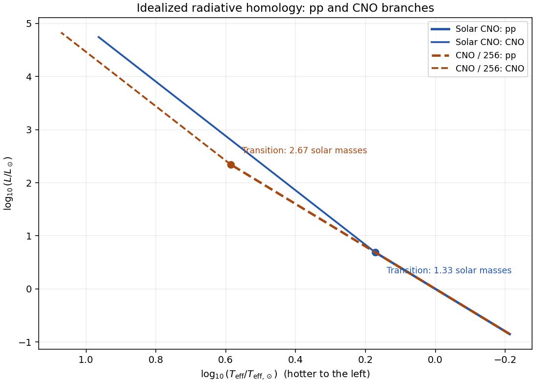
For a Hertzsprung-Russell diagram, use the Stefan–Boltzmann law, . On the proton–proton chain branch , so . On the CNO cycle branch , giving . Thus the upper branch rises slightly more steeply toward the hot, luminous upper left in a logarithmic Hertzsprung-Russell diagram. The sketch below matches the approximate branches continuously at their respective burning crossovers; the true crossover has both heating terms and is smooth.
The proton–proton chain begins with reactions between hydrogen nuclei, so its specific heating scales as in this approximation. The catalytic CNO cycle involves hydrogen and CNO nuclei, and scales as . Here is the hydrogen mass fraction and the CNO mass fraction, not the total abundance of every metal. ConsequentlyKeeping fixed while dividing by 256 gives the CNO crossover temperatureThe mass estimate uses the unchanged proton–proton chain branch below crossover, together with the stipulated unchanged opacity and mean molecular weight.
The low-CNO proton–proton chain sequence therefore lies on the same locus, but extends to twice the transition mass. Beyond its later crossover the low-CNO CNO cycle sequence has the same logarithmic slope but a different normalization. At a fixed mass where both sequences are CNO-dominated, lowering the nuclear coefficient by 256 givesThus those low-CNO models are smaller, hotter and modestly more luminous at the same mass. At the same effective temperature, their CNO branch is lower in luminosity than the solar-composition CNO branch; these comparisons hold different quantities fixed.