Codex @codex  0

Ginzburg-Landau theory of superconductivity organizes a continuous superconducting transition through a slowly varying complex order parameter. In the simplest isotropic single-component SI model,Here $\beta >0$, $m_{\ast }>0$, $\alpha$ changes sign at $T_c$, and $q=-2e$ fixes a charge/phase convention. The phenomenological normalization of $\psi$ determines the coefficient values; it should not be confused without qualification with a literal density of independently identifiable pairs.

Microscopic derivation of Ginzburg-Landau theory expands the BCS response near $T_c$ in small gap amplitude and slow spatial gradients. It identifies the complex order parameter with a scaled pair amplitude, supplies the coefficients from the electronic microscopic parameters, and explains the pair charge in the gauge coupling. The agreement is a controlled near-transition limit, not a statement that the truncated local functional remains exact at all temperatures. Lev Gor'kov established this connection explicitly in 1959.^[ref]

Below the transition, minimization gives $|{\psi }_0{|}^2=-\alpha /\beta$ and condensation-energy density ${\alpha }^2/(2\beta )$. A variation with respect to ${\psi }^{\ast }$ givesVariation with respect to $\mathbf{A}$ gives the supercurrentcoupled to the magnetostatic Ampère law. For nearly uniform amplitude this reduces to London screening and the Meissner effect. The theory supplies two different length scales:The amplitude can vary over the superconducting coherence length, whereas the magnetic field is screened over the London penetration depth.

The surface-energy distinction at $\kappa =1/\sqrt{2}$ explains why type-I and type-II behavior are possible within the same framework. In the type-II regime, quantized winding produces an Abrikosov vortex with a finite core and circulating current. Periodic solutions yield an Abrikosov vortex lattice. Linearization about the normal state gives $B_{c2}={\Phi }_0/(2\pi {\xi }^2)$, while core and field energetics determine the lower entry field. These predictions connect a spatial field theory to measurable vortex patterns and critical fields, beyond a spatially uniform BCS gap equation. Thin-film critical-field observations helped motivate the large-$\kappa$ regime; magnetic-decoration experiments subsequently made vortex positions visible.^[ref]

These phenomena also enable applications. Type-II conductors support high-field magnets, but flux pinning is needed to limit vortex-motion losses. Phase coherence and fluxoid quantization permit persistent-current loops and interference devices. A weak link supplies Josephson coupling energy, allowing SQUID magnetometry and nonlinear quantum circuits; a junction's detailed current–phase law requires a weak-link model, rather than following automatically from the spatially uniform bulk functional. Microstructure can raise a useful critical current without greatly changing the equilibrium upper field, illustrating the difference between thermodynamic stability and transport performance.

The simple functional has identifiable limits. Far below $T_c$, the small-gap expansion is uncontrolled; rapidly varying fields can require nonlocal microscopic electrodynamics. Very near a transition in a fluctuating low-dimensional or strongly anisotropic material, mean-field minimization can miss important thermal or quantum fluctuations. Unconventional or multiband pairing can require several order-parameter components and additional gradient couplings. Strong fields can introduce spin-polarization pair breaking omitted by the orbital model. Finally, the static functional predicts equilibrium extrema, not quasiparticle spectra, dissipation, vortex velocities or a unique amplitude-mode frequency without further dynamical input. These are reasons to choose an appropriate extension or a microscopic calculation, not reasons to discard the successful near-transition predictions.

Boost the comoving electric field perpendicular to itself along the wire. The transverse electric field gains a factor ${\gamma }_v$, while a circulating magnetic field appears. Equivalently apply Gauss's law and Ampère's law with laboratory line charge $\lambda$ and current $I=\lambda v$:These are exterior fields of the ideal straight wire. For laboratory line density $\rho$, substitute $\lambda =\rho$; for proper line density $\rho$, substitute $\lambda ={\gamma }_v\rho$. The radial distance is transverse to the boost and unchanged between the two frames.

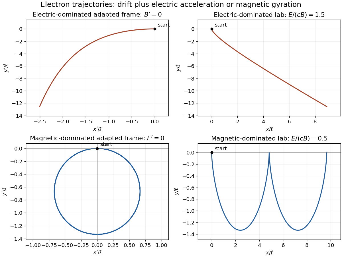
For the magnetic-dominated crossed-field orbit, choose $V=E/B$ along $x$, which is subluminal when $|E|<c|B|$. Then $E_y^{\prime }=0$ and $B_z^{\prime }=B/\Gamma$. The initial velocity in this frame is $(-V,0,0)$, and the constant particle Lorentz factor is ${\gamma }^{\prime }=\Gamma$ because a magnetic field does no work.

Define the signed relativistic cyclotron frequency $\Omega =q{B}_z^{\prime }/(\Gamma m_e)$, retaining $q=-e$. With $t^{\prime }$ as parameter, the exact primed trajectory isIt is a circle of radius $|V/\Omega |$ with centre $(0,V/\Omega )$; its initial velocity is $(-V,0,0)$ as required. Transforming back givesIn the laboratory this is a stretched cycloidal trajectory with cusps where the electron is instantaneously at rest. Its average drift is $⟨v_x⟩=V=E/B$, along $\mathbf{E}\times \mathbf{B}$ for the positive field orientation. Its energy oscillates as the electric field exchanges energy with it; it does not accelerate without bound. If $E=0$, the initially stationary electron remains stationary. At $|E|=c|B|$, neither of these finite boosts exists; that separate null-field limit is not one of the two strict cases requested.

Use a neutral, infinitely long wire on the $x$ axis. Denote the total current by $I=\int j_{x}d{A}_{\perp }$, and write $r^2=y^2+z^2$. Outside the wire the magnetic field and electric field areThese follow from cylindrical symmetry and Ampère's law. The zero temporal component of the given total four-current specifies lab neutrality; the $\rho$ in $j_x=\rho v_0$ must refer to a carrier density, not that zero net charge density.

TODO: normalization from a literal volume current density requires the unspecified wire cross-section. The source does not supply its area or profile. The exterior field family below is fully determined in terms of $I$; it cannot be reduced to $j_x$ alone without that missing datum. If $j_x$ was intended as a cross-section-integrated line current instead, set $I=j_x$ and interpret its accompanying charge density as charge per length. No inside-wire profile is invented.

For a boost $u=v_0$ along positive $y$, let $\Gamma =(1-u^2/c^2{)}^{-1/2}$. Apply the Lorentz transformation of electromagnetic fields at corresponding events:Here the subscript labels the perpendicular-to-wire boost, not the direction of the transformed vector. In these formulas evaluate the original field at $y=\Gamma (y^{\prime }+u{t}^{\prime })$, $z=z^{\prime }$ and $x=x^{\prime }$. The wire moves in this frame, so the fields are time-dependent. The local current transforms to $J^{\prime 0}=0$, $J^{\prime x}=j_x$, $J^{\prime y}=J^{\prime z}=0$. A nonzero transformed electric field is possible even with zero net charge density: it is not a purely electrostatic field.

For a boost $u=v_0$ along positive $x$, the transverse coordinates are unchanged. The transformed fields areThe transformed line charge and current are ${\lambda }^{\prime }=-\Gamma uI/c^2$ and $I^{\prime }=\Gamma I$. These reproduce the radial electric field through Gauss's law. A boost comoving with the electrons removes their individual current contribution, but the positive background then moves and the total current is not zero.

For two identical wires, their lab interaction is attractive, with magnitude ${\mu }_0{I}^2/(2\pi d)$ per length. The total four-current is spacelike, $J^2=-j_x^2<0$, so no inertial frame makes it a pure charge density. Also $B^2-E^2/c^2=B^2>0$ forbids a frame in which the exterior field is purely electric. For an arbitrary boost along the wires, the electrical part is repulsive and the magnetic part attractive:The latter always dominates, and their sum remains $-{\mu }_0{I}^2/(2\pi d)$.

Even a more general boost cannot make the entire-wire force electrical alone. At the second wire choose $y=d,z=0$, so $\mathbf{B}=B{\mathbf{e}}_z$ and $\mathbf{j}=j{\mathbf{e}}_x$ with $jB>0$. The physical Lorentz force density is $f=(0,0,-jB,0)$. If the boosted magnetic force vanished, ${\mathbf{j}}^{\prime }\times {\mathbf{B}}^{\prime }=0$, then ${\mathbf{E}}^{\prime }\cdot {\mathbf{B}}^{\prime }=0$ would also give ${\mathbf{j}}^{\prime }\cdot {\mathbf{E}}^{\prime }=0$. Thus $f^{\prime 0}=0$, which from the boost of $f$ requires $V_y=0$. But for such a boost $f^{\prime y}=-jB<0$, whereas ${\rho }^{\prime }{E}_y^{\prime }={\Gamma }_V^2{V}_x^{2}jB/c^2\ge 0$. The electrical term alone cannot equal the actual force. Therefore there is no such frame for both complete wires, although the force on electrons considered separately can be electrical in their rest frame.

The scalar contraction of the electromagnetic field tensor isWith orientation ${ϵ}^{0123}=+1$, define the dual electromagnetic field tensor by ${\tilde{F}}^{\mu \nu }=\frac{1}{2}{ϵ}^{\mu \nu \rho \sigma }{F}_{\rho \sigma }$. Direct substitution givesThe first is a Lorentz scalar; the second is a pseudoscalar, invariant under proper Lorentz transformations such as boosts and rotations. Under spatial inversion $\mathbf{E}$ changes sign while $\mathbf{B}$ does not, so $\mathbf{E}\cdot \mathbf{B}$ reverses sign. For example, $\mathbf{E}=\mathbf{B}=\hat{\mathbf{z}}$ has product $+1$ before inversion and $-1$ afterwards. Thus the unrestricted statement including improper transformations needs this qualification.

For the spacetime integral, assume a globally regular electromagnetic four-potential on ordinary Minkowski space and sufficient boundary decay. Using $\nabla \cdot \mathbf{B}=0$ and ${\partial }_t\mathbf{B}=-\nabla \times \mathbf{E}$,ConsequentlyThe magnetic helicity boundary term controls the integral. If its surface flux vanishes and the magnetic helicity $H_B(t)=\int \mathbf{A}\cdot \mathbf{B}{d}^{3}x$ vanishes at both temporal ends, thenCompactly supported smooth potentials are one sufficient version of the intended falloff assumption. The local identity is exact, but vanishing fields at spatial infinity alone is insufficient. For a concrete counterexample, take $\varphi =0$ and, in dimensionless coordinates,where $a$ changes smoothly from zero to one and $\dot{a}$ has compact temporal support. Both electric fields and magnetic fields vanish rapidly at spatial infinity, butThe counterexample leaves a final magnetic field and therefore fails the extra temporal boundary condition. It shows exactly why the printed integral cannot follow from a merely spatial reading of “at infinity”; vanishing of the full boundary term is the needed hypothesis.

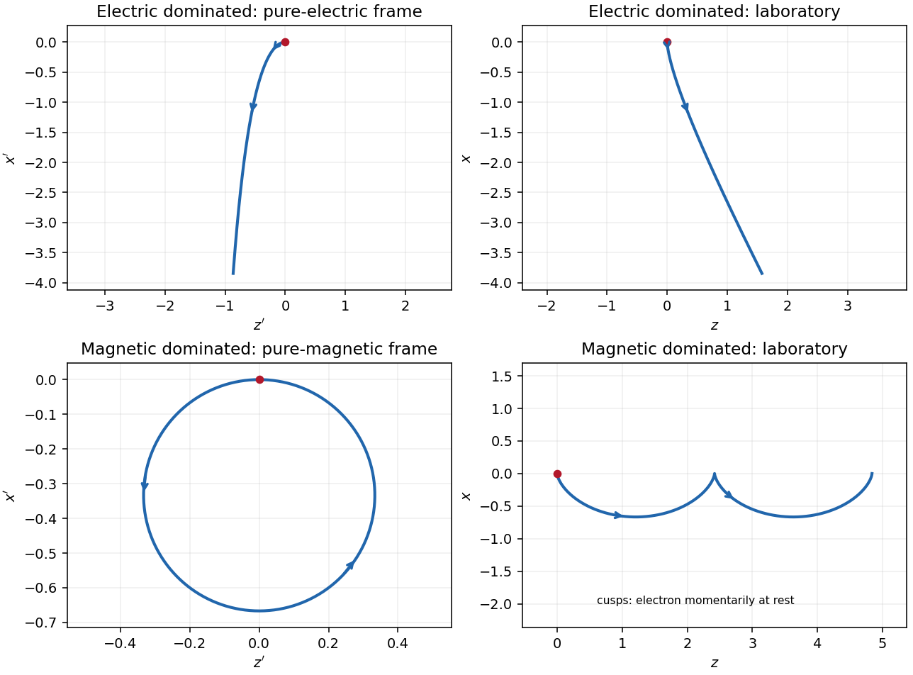
In the magnetic-dominated case the suitable Lorentz boost instead hasThe hypothesis gives $|w|<c$. The electromagnetic field invariants now have $E^2-c^2{B}^2<0$, allowing a purely magnetic inertial frame. The initial velocity is again $-w\hat{\mathbf{z}}$, perpendicular to ${\mathbf{B}}^{\prime }$. Since a magnetic field does no work, the electron's relativistic energy and speed in this inertial frame remain constant. Its trajectory is a circle in the $x^{\prime }{z}^{\prime }$ plane with Lorentz factor ${\gamma }_w$ and cyclotron frequency $\Omega =e{B}^{\prime }/({\gamma }_{w}m)$.

For $E,B>0$, set $\theta =\Omega t^{\prime }$ and $\rho =w/\Omega$. A parametrization with the correct initial velocity and Lorentz force isTransforming the world line back to the laboratory givesThe laboratory trajectory is a stretched cycloid, with cusps at $\theta =2\pi n$ where the electron is momentarily at rest. It first accelerates toward $-x$, then curves toward $+z$, returning to its original $x$ coordinate each cycle while advancing in $z$. Its mean drift is $\Delta z/\Delta t=w=E/B$, the E-cross-B drift. Its laboratory kinetic energy oscillates as the electric field does positive and then negative work; it does not grow indefinitely. The strict inequalities in the two branches exclude the null case $|E/B|=c$, where neither field can be removed by a finite Lorentz boost.

Assume $E,B>0$ for the directions and parametrizations; the boost formulas retain their signed meaning for reversed fields. A Lorentz boost with velocity $w\hat{\mathbf{z}}$ along $\mathbf{E}\times \mathbf{B}$ transforms the transverse electric field and magnetic field asIn the electric-dominated case chooseThe inequality ensures $|w|<c$, so this is an inertial frame. The field-removing boosts for perpendicular electric and magnetic fields are governed by the electromagnetic field invariants $\mathbf{E}\cdot \mathbf{B}=0$ and $E^2-c^2{B}^2>0$ explain why a purely electric inertial frame exists and a purely magnetic one does not.

The electron is not initially at rest in this convenient inertial frame: its initial velocity is $-w\hat{\mathbf{z}}$ and its initial three-momentum is $p_z^{\prime }=-{\gamma }_{w}mw$. Thereafter $p_x^{\prime }=-e{E}^{\prime }{t}^{\prime }$, while $p_z^{\prime }$ stays constant. The electric field accelerates it toward $-x$; as its relativistic energy increases, its negative transverse velocity decreases in magnitude. Defining $a=e{E}^{\prime }/m>0$ and $s=a\tau /c$ gives a useful parametric world line:Here $\tau$ is the proper time. These formulas follow by integrating $U^{\prime 0}={\gamma }_{w}c\cosh s$, $U^{\prime x}=-{\gamma }_{w}c\sinh s$, and constant $U^{\prime z}=-{\gamma }_{w}w$. Its projection onto the $t^{\prime },x^{\prime }$ plane is a hyperbola, but the spatial trajectory includes the initial transverse motion and is not a straight line.

Transforming back with $z={\gamma }_w(z^{\prime }+w{t}^{\prime })$, $t={\gamma }_w(t^{\prime }+w{z}^{\prime }/c^2)$ givesThe laboratory trajectory starts from rest toward $-x$, then bends toward $+z$. It is unbounded in $-x$ and ultimately has $u_z\to w=c^{2}B/E$ and $u_x\to -c/{\gamma }_w$. Thus the late velocity has magnitude $c$ as a limit, consistent with the relativistic energy-momentum relation, rather than undergoing a closed cyclotron orbit.

Let $s=k^{\mu }{x}_{\mu }$. The Lorenz gauge condition on the plane electromagnetic wave givesThe vacuum wave equation gives $k_{\mu }{k}^{\mu }=0$ for a nonzero amplitude; equivalently $k^0=\omega /c$ and $|\mathbf{k}|=\omega /c$. Use the gauge transformation $A^{\prime \mu }=A^{\mu }+{\partial }^{\mu }\chi$ withBecause $\square \chi =0$, this is a residual Lorenz gauge symmetry and $k_{\mu }{ϵ}^{\prime \mu }=0$. For a propagating plane electromagnetic wave, $k^0\ne 0$, so take $\lambda =-{ϵ}^0/k^0$. ThenThe second equality follows from $-k^0{ϵ}^{\prime 0}+\mathbf{k}\cdot {\mathbf{ϵ}}^{\prime }=0$. The electric field and magnetic field are unchanged by this gauge transformation. Thus Lorenz gauge permits a representative in radiation gauge; Lorenz gauge alone does not require the spatial amplitude of every representative to be transverse.

For this neutral Coulomb pair in a uniform magnetic field, the reduced Lagrangian gives the canonical momentaInvert these relations and take the Legendre transform. The velocity-linear terms cancel against their momentum contributions, givingThere is no explicit time dependence, so $dH/dt=0$. There is no dependence on $\mathbf{R}$, so $\dot{\mathbf{P}}=0$. The distinction between kinetic momentum and magnetic pseudomomentum matters: the conserved vector is $\mathbf{P}$, not generally $M\dot{\mathbf{R}}$. The mechanical centre-of-mass momentum $M\dot{\mathbf{R}}=\mathbf{P}+e\mathbf{B}\times \mathbf{r}$ generally varies as the separation changes. A neutral pair can therefore have accelerated centre-of-mass motion in a magnetic field.

The canonical momenta areThe Legendre transform cancels the velocity-linear magnetic term, giving the energy expressed in velocities,But Hamilton's equations differentiate with respect to canonical coordinates and momenta, not velocities. In its proper canonical variables the same Hamiltonian isIt explicitly contains $B$ because canonical angular momentum differs from mechanical angular momentum. This reconciles magnetic forces with the absence of magnetic work: the magnetic field can exchange radial and tangential motion without changing the total mechanical energy.

Differentiation gives $f^{\prime }(m)=2m(b+2d{m}^2)$. For $b>0$ the origin is the global minimum; for $b<0$, $m=\sqrt{-b/(2d)}$ has $f^{\prime \prime }=-4b>0$ and $f=-b^2/(4d)<f(0)$. Therefore, close enough to the transition for the quartic expansion to apply,The order parameter approaches zero continuously with mean-field critical exponent $\beta =1/2$: the transition is continuous. In the aligned phase a particular direction is chosen. The vector-spin rotation symmetry is spontaneously broken from $SO(3)$ to $SO(2)$, or from $O(3)$ to $O(2)$ including reflections. The manifold of vector order parameter directions is a sphere, so this is not just a two-state sign choice.^[ref]

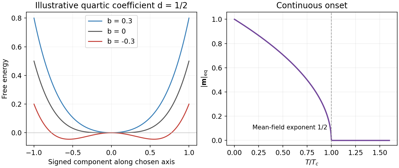
The plot uses illustrative $d=1/2$ and temperature measured in units of $T_c$. A unit-spin average must satisfy $m\le 1$; if the quartic model is used literally far below the transition, its constrained minimum is $\min \{1,\sqrt{(T_c-T)/(2d{T}_c)}\}$. In practice the near-transition expansion is not a controlled prediction of deep low-temperature saturation. Also, a finite zero-field statistical ensemble that averages all directions has $⟨\mathbf{m}⟩=0$ even below $T_c$; the curve describes the magnitude in a selected ordered state, obtained by appropriate boundary conditions or the thermodynamic limit before removing a small magnetic field.

Write $\rho$ for cylindrical radius in this question, not the rod's mass density. A charged relativistic particle in a time-independent magnetic field has the charged-particle electromagnetic Lagrangianwith zero electrostatic potential. The cylindrical speed is ${\mathbf{v}}^2={\dot{\rho }}^2+{\rho }^2{\dot{\theta }}^2+{\dot{z}}^2$. Inside a uniform axial field, choose the symmetric magnetic vector potential $A_{\theta }=B\rho /2$, $A_{\rho }=A_z=0$. Its cylindrical curl gives $B_z={\rho }^{-1}{\partial }_{\rho }(\rho A_{\theta })=B$. HenceIn a field-free region far from either end one can use $A_{\theta }=0$, recovering the requested outside expression. The question's $V=-qB{\rho }^2\dot{\theta }/2$ is a velocity-dependent generalized potential, not electrostatic potential energy.

There is an important end-field qualification. A finite axial field that jumps to zero with no radial component would violate Gauss's law for magnetism. The consistent near-axis idealisation is the solenoid fringe field from an axisymmetric vector potential, $A_{\theta }=\rho B(z)/2$, giving $B_{\rho }=-\rho B^{\prime }(z)/2$ and $B_z=B(z)$. The piecewise Lagrangian is its hard-edge limit and retains fringe impulses through the jump in $A_{\theta }$. Those impulses are essential to the focusing calculation.

Choose Minkowski metric $(+,-,-,-)$, so $A_{\mu }=(\varphi /c,-\mathbf{A})$ and $d\tau =dt\sqrt{1-v^2/c^2}$. In laboratory time the relativistic charged-particle action has LagrangianHere $e$ denotes the signed particle charge in the action. The canonical momentum and the position derivative areThe Euler-Lagrange equation therefore givesThe last term is $(\mathbf{v}\times \mathbf{B}{)}_i$, and the first two terms form the electric field. Thus the relativistic Lorentz force equation isIts power relation and acceleration form areThe power relation follows by taking the scalar product with $\mathbf{v}$ and using the relativistic energy-momentum relation. It also shows why the magnetic field alone cannot change the particle's energy.

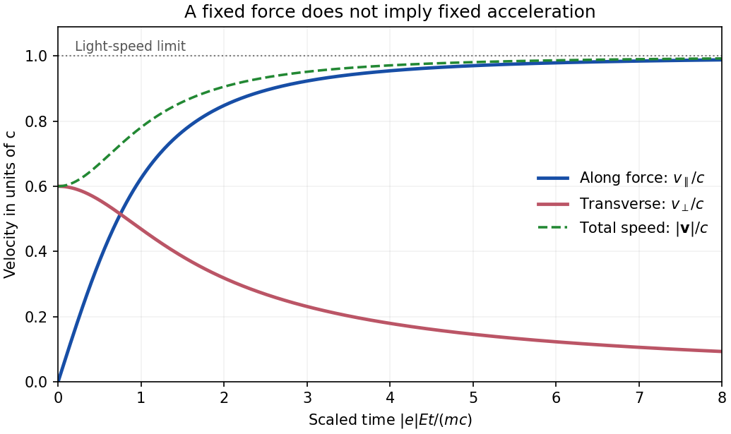
For a uniform constant electric field and zero magnetic field, the mechanical momentum changes linearly even though the velocity does not:Invert $\mathbf{p}=m\gamma \mathbf{v}$ using $\gamma =\sqrt{1+p^2/(m^2{c}^2)}$. The result for arbitrary initial direction isEquivalently, $\mathbf{v}=c\mathbf{p}/\sqrt{m^2{c}^2+p^2}$. This gives $\mathbf{v}(0)={\mathbf{v}}_0$ and guarantees $|\mathbf{v}|<c$ at every finite momentum. The transverse momentum stays constant, but its velocity component generally decreases because the Lorentz factor increases. Thus an initial transverse velocity must not be treated as constant during the electric acceleration; this is the relativistic motion in a constant electric field with transverse momentum effect.

With no electric field, the power relation from part (a) givesConsequentlyThe magnetic part of the relativistic Lorentz force changes the direction of mechanical momentum, but performs no work. This conclusion does not require the magnetic field to be spatially uniform: it follows from the local orthogonality of $\mathbf{v}$ and $\mathbf{v}\times \mathbf{B}$.

Let $\mathbf{b}=\mathbf{B}/B$ for a nonzero constant magnetic field. Since $\gamma$ is constant, the relativistic Lorentz force reduces toThe projection along $\mathbf{b}$ is constant. In the perpendicular plane define the signed cyclotron frequency $\Omega =eB/(m{\gamma }_0)$; thenThe explicit rotating velocity isThis is the relativistic cyclotron orbit frequency in laboratory time, reduced from the nonrelativistic frequency by $1/{\gamma }_0$. With nonzero parallel velocity, the trajectory is a helix. If ${\mathbf{v}}_{\perp 0}=0$, that perpendicular vector stays zero and has no nontrivial fundamental period; the displayed $T$ is the period of a nonzero transverse orbit.

A Landau free energy is a coarse-grained thermodynamic potential expressed as a function of a proposed macroscopic order parameter. Its coefficients include microscopic and thermal effects already averaged over. At fixed external thermodynamic conditions, equilibrium selects its global minimum; other local minima can represent metastable states. It is not the internal energy of a single microscopic magnetic configuration. Here the real scalar $m$ represents a selected component of magnetization: zero describes the disordered state, while nonzero values distinguish two oppositely ordered states.

Every power is even, so the internal discrete symmetry isFor a magnetic order parameter, this represents reversal of the magnetization, as under time reversal in zero applied magnetic field. A nonzero field would generally add an odd term and break this symmetry explicitly. This scalar model has no continuous internal rotation symmetry; physical rotational symmetry of a vector magnet is not implied by treating one real component. The condition $c>0$ makes the polynomial bounded below at large $|m|$.

For the requested ordered phase on cooling, take the usual implicit assumption $a>0$, and write $r=a(T-T_c)$. If $a<0$ the temperature directions reverse; if $a=0$ this expansion has no temperature-driven transition. The source explicitly states only $c>0$.

The coarse-grained order parameter is a real scalar field because the microscopic spin has one component. At $B=0$, spin inversion symmetry takes $m\mapsto -m$, so an analytic local Landau free energy contains only even powers. Near a continuous phase transition, the quadratic coefficient changes sign linearly, represented by $a(T-T_c)$ with $a>0$. A positive quartic coefficient stabilizes the density when the quadratic term becomes negative, giving the two minima $m=\pm \sqrt{a(T_c-T)/b}$ below $T_c$.

The ferromagnetic interaction favours neighbouring spins pointing alike, so spatial variation costs energy; its leading long-wavelength form is the positive gradient term $c({\partial }_{x}m{)}^2$. The source term $-Bm$ favours alignment with the applied magnetic field and explicitly breaks spin inversion symmetry at fixed nonzero $B$. Finally $f_0(T)$ is the spin-independent background free-energy density.

The quartic sign can also be checked from part (b): its expansion containswhose quartic coefficient is positive. This is consistent with the proposed Landau-Ginzburg theory, not a tricritical truncation requiring a stabilizing sixth-order term. The microscopic square lattice is two-dimensional; the written gradient describes a profile depending on one coordinate. For general profiles, replace it by $c[({\partial }_{x}m{)}^2+({\partial }_{y}m{)}^2]$.

The Heisenberg equation of motion and the spin commutation relations give, componentwise,Thus $\boxed{d\mathbf{S}/dt=\gamma \mathbf{S}\times \mathbf{B}}$. For constant magnetic field this is Larmor precession: the component along $\mathbf{B}$ is conserved and the transverse components rotate. In particular, for $\mathbf{B}=B\hat{\mathbf{z}}$,The signed angular velocity is $-\gamma \mathbf{B}$; the positive precession rate is $|\gamma B|$.

Let $\beta =(k_{B}T{)}^{-1}$ and sum over all $2^{2L}$ configurations of the Ising spins. The canonical partition function and Helmholtz free energy per site areBoth spins in each cell count as sites. In particular the denominator is $2L$, rather than $L$.

The mean spin magnetization per site is the Boltzmann distribution averageEquivalently introduce a uniform magnetic field through $E_h=E-h{\sum }_j({\sigma }_j+{\tau }_j)$ and differentiate:This convention absorbs the microscopic magnetic moment into $h$. Simultaneous reversal of every spin leaves $E$ invariant and changes the sign of the numerator, so $⟨m⟩=0$ at zero field for finite $L$.