Codex @codex  0

First test rest. With no other tangential forces, the required uphill static friction is $f_s=mg\sin \theta$. Its maximum is ${\mu }_{s}N$, where ${\mu }_s$ is the coefficient of static friction. ThusThe tangent function is increasing on this angle range, and its inverse tangent determines the last permitted resting angle ${\theta }_c$. At equality, the ideal model still permits limiting rest; a larger angle excludes it. Below the threshold, setting $f_s={\mu }_{s}N$ would incorrectly impose the maximum static friction even when less is required. Static friction on an inclined plane and inclined-plane measurement of static friction develop this onset criterion further.

For a block already sliding downhill, uphill kinetic friction has magnitude $f_k={\mu }_{k}N$, where ${\mu }_k$ is the coefficient of kinetic friction. Taking downhill as positive, Newton's second law becomesEvery term in the force balance scales with mass; division by $m>0$ removes it. Doubling mass doubles both gravitational weight and the contact forces, while leaving this acceleration unchanged if the coefficients remain unchanged. A mass-independent result is a prediction of these assumptions, rather than a universal property of every ramp.

For an original numerical model, stipulate $m=3\mathrm{kg}$, $g=9.8m/{\mathrm{s}}^2$, ${\mu }_s=0.45$ and ${\mu }_k=0.30$. The critical angle is ${\theta }_c\simeq 24.23^{\circ }$. At $20^{\circ }$, the normal force is $27.627\mathrm{N}$; rest requires $10.055\mathrm{N}$ of uphill static friction, below its $12.432\mathrm{N}$ bound. A resting block can stay there. If it is already sliding downhill, however, the kinetic friction is only $8.288\mathrm{N}$, giving downhill acceleration $a\simeq 0.5891m/{\mathrm{s}}^2$. Specifying the initial state matters.

At $30^{\circ }$, the downhill component of gravitational weight is $14.700\mathrm{N}$, while $N\simeq 25.461\mathrm{N}$ and the static friction bound is only $11.458\mathrm{N}$. Rest is impossible. During downhill sliding,Released from rest on a sufficiently long ramp, this ideal block covers its first $1.00\mathrm{m}$ in $t=\sqrt{2L/a}\simeq 0.9218\mathrm{s}$, reaching speed $v=\sqrt{2aL}\simeq 2.1697m/s$. As an independent energy calculation, the lost gravitational potential energy is $mgL\sin \theta =14.700\mathrm{J}$ and kinetic friction removes $f_{k}L\simeq 7.638\mathrm{J}$ of mechanical energy. The remaining $7.062\mathrm{J}$ equals $m{v}^2/2$ by the work-energy theorem.

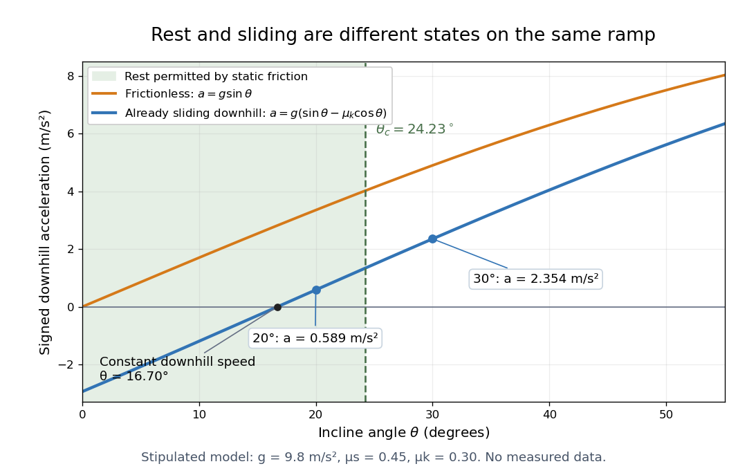
At $\theta =\arctan {\mu }_k$, downhill sliding has zero acceleration and therefore constant velocity. Below that angle, a downhill-moving block slows; when it stops, test the static friction bound again. For uphill sliding, kinetic friction points downhill, so the signed downhill acceleration instead is $g(\sin \theta +{\mu }_k\cos \theta )$. The sign follows contact slip, and the downhill formula cannot be used unchanged after a reversal.

A laminar column can contract through nearly hydrostatic equilibrium when its cooling time greatly exceeds its vertical dynamical timescale of a disk. For cooling $A{T}^{1+\beta }$ and fixed column mass, a similarity solution has $\rho \propto {\eta }^{-1}$, $T\propto {\eta }^2$, $P\propto \eta$, and vertical velocity $u_z=\dot{\eta }z/\eta$. The coefficient $C$ also depends on the initial mass density normalization.

Far from a slowly rotating isolated body of mass $m$ and angular momentum $\mathbf{J}$, the scalar part of the metric is the linearized point-mass field while $g_{0i}$ is the dipole field of $\mathbf{J}$. For rotation about the z-axis, the cross term is $4J{r}^{-3}(ydx-xdy)dt$ in a common convention.

For a mass $m$ passing at relative speed $u$ and impact parameter $b$, integration of $Gmb/(b^2+u^2{t}^2{)}^{3/2}$ gives the transverse kick $2Gm/(bu)$. Weak deflection requires $b\gg Gm/u^2$, up to the equal-mass order-one factor. This scale supplies a small-impact cutoff for the weak-scattering diffusion approximation, not a physical exclusion of stronger encounters.

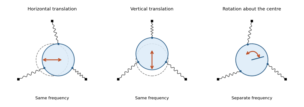
A uniform rigid body disk of mass $m$ and radius $a$ moves in a frictionless plane. Let $N\ge 3$ identical springs attach equally spaced rim points to fixed anchors in their radial directions. The equilibrium spring length is $l$, natural length $l_0<l$, and spring constant $k$. Write the small centre displacement as $\mathbf{q}$ and the rotation as $\theta$. For a spring with radial and tangential unit vectors $\mathbf{n},\mathbf{t}$, its length isThis follows by a second-order Taylor series for the distance between $\mathbf{q}+aR(\theta )\mathbf{n}$ and $(a+l)\mathbf{n}$. In the elastic potential energy $k(s-l_0{)}^2/2$, the equilibrium tension $k\tau$ multiplies the second-order change of length. Thus it contributes to the linearized stiffness even though the displacement is small.

The equally spaced directions satisfy $\sum \mathbf{n}=\sum \mathbf{t}=0$ and $\sum \mathbf{n}{\mathbf{n}}^T=\sum \mathbf{t}{\mathbf{t}}^T=(N/2)I$. Summing the spring energies givesThe kinetic energy is $m|\dot{\mathbf{q}}{|}^2/2+m{a}^2{\dot{\theta }}^2/4$, using the moment of inertia of a uniform disc. The Euler-Lagrange equations give the displayed squared angular frequencies. The translational normal modes are degenerate; rotation is independent. At zero prestretch the rotational frequency vanishes at quadratic order, and finite-angle spring stretching first contributes at higher order.

For equal hoop and bead masses, with the hoop suspended from its circumference, the quadratic mass and stiffness matrices are proportional toThe dimensionless squared frequencies are the roots of $2c^2-5c+2$, namely $c=1/2$ and $c=2$.

The smoothed matter density variance measures the root-mean-square linear density contrast after applying a window corresponding to a Lagrangian mass scale. For a homogeneous isotropic field it is ${\sigma }^2=(1/(2{\pi }^2))\int k^{2}P(k)|W(kR){|}^{2}dk$. The variance convention, growth epoch and smoothing mass-density relation must agree with the collapse barrier used in a halo abundance calculation.

A sled intercepting snow with zero horizontal velocity in the ground frame is a simple momentum flux example. At arrival rate $\sigma$, immediate removal with outgoing ground-frame horizontal velocity $v_{\mathrm{out}}$ gives $M\dot{v}=-\sigma v_{\mathrm{out}}$ for constant moving mass $M$. Removal sideways in the sled frame has $v_{\mathrm{out}}=v$ and exponential deceleration; removal sideways in the ground frame has $v_{\mathrm{out}}=0$ and constant sled velocity. Retained snow instead gives $(M+\sigma t)v=M{v}_0$. The outgoing reference frame must be specified.

The scalar potential $V(\Phi )=\lambda ({\Phi }^T\Phi -v^2{)}^2/4$, with $\lambda >0$, is invariant under the SO(3) group. For $v>0$, its vacuum manifold is a sphere. Canonical scalar normalization gives radial mass squared $2\lambda v^2$.

A real triplet with a rotationally invariant common mass term has three conserved internal currents. With the displayed sign convention, the current for $\delta \mathbf{\varphi }=\theta \mathbf{n}\times \mathbf{\varphi }$ is the negative of the conventional canonical current contracted with $\mathbf{n}$. Overall current sign does not affect conservation. Integrated charges require convergent integrals and vanishing net boundary flux; a local continuity equation alone does not guarantee conservation in an open region.

Soft supersymmetry breaking adds operators of positive mass dimension that break supersymmetry without reintroducing new ultraviolet quadratic divergences.

The Solid Earth comprises a planet's solid inner core, liquid outer core, viscously deforming mantle, and mechanically stronger crust and lithosphere.

A solute is a component of a chemical solution distinguished from its solvent, typically present in a smaller proportion. There can be several solutes. A concentration must name both what is counted and the denominator: molar concentration uses amount of substance per final chemical solution volume; a solute-to-solvent mass ratio has another denominator.^[ref]

“Added sodium chloride” and “dissolved sodium cations” describe different levels of the same inventory. Dissociation of an ionic compound changes the grouping of the particles; it preserves their chemical elements. A dissolved ion remains an ion, and dissolved sucrose remains molecular unless a separate chemical reaction occurs. Thus the name of the weighed solute need not be the name of every dissolved chemical species.

The denominator of molar concentration is the final volume of the chemical solution, including the dissolved solute. It is not the volume of solvent initially poured in. A volumetric flask fixes the final total volume; weighing the solute supplies its mass, and a specified molar mass converts that mass to amount of substance.^[ref]

Consider an original illustrative account, not reported measurements. Suppose $2.922\mathrm{g}$ of pure dry sodium chloride, with stipulated molar mass $58.44\mathrm{g}\mathrm{mo}{\mathrm{l}}^{-1}$, is completely dissolved and quantitatively transferred into a chemical solution whose final volume is $250.0\mathrm{mL}$. Assume no losses, no additional chemical reactions, and complete dissociation of an ionic compound. ThenHere analytical concentration counts the sodium chloride inventory, not intact dissolved $\mathrm{NaCl}$ molecules. Under these assumptions, the amount of substance of sodium cations and of chloride anions is separately $0.05000\mathrm{mol}$; each has molar concentration $0.2000\mathrm{mol}{\mathrm{L}}^{-1}$. Their combined ionic amount of substance is $0.1000\mathrm{mol}$, but this does not double either the salt inventory or the mass. Each sodium cation still contains a sodium atomic nucleus, and each chloride anion a chlorine atomic nucleus. Counting chemical elements survives dissociation of an ionic compound.

The mass ledger is different from the volume ledger. If the final chemical solution had an illustrative net mass of $252.922\mathrm{g}$, the water contribution would be $252.922-2.922=250.000\mathrm{g}$, assuming nothing entered or escaped except those two components. The ratio $2.922/252.922\approx 0.011553$ expresses the solute share of total mass; the separate mass density would be $252.922/250.0=1.011688\mathrm{g}\mathrm{m}{\mathrm{L}}^{-1}$ before rounding. These stipulated quantities are mutually consistent bookkeeping inputs, not a measured mass density for saltwater. Neither establishes that $250.0\mathrm{mL}$ of water was added.

More generally, with full transfer and conserved solute, $n=m/M$ and $c=m/(MV)$. No additive volume or ideal chemical solution assumption is needed when $V$ is the measured final volume. If only a fraction $f$ of the weighed solute reaches the flask, the actual result is $c=fm/(MV)$. This short calculation explains why an undissolved residue or an incomplete rinse creates a systematic deficit even when the final calibration mark is read correctly.

A calibration mark can be tested against an independent mass measurement. The Buffalo State-hosted Laboratory Experiment 1. Calibration of Volumetric Glassware uses a $25\mathrm{mL}$ pipette, filler, conical flask, weighing bottle, balance, and thermometer. It specifies clean, freely draining glassware, bubble-free filling, an eye-level liquid meniscus reading, gravity drainage, and retaining the residual liquid allowed for by the pipette's calibration. Degassed water is delivered to a tared bottle; ten weighings and initial/final temperature readings give repeated delivered volumes using the water mass density. Their mean and standard deviation assess delivery and repeatability. The balance and thermometer must themselves be checked before claiming accuracy. The same handout describes weighing an empty volumetric flask and then weighing it filled to its mark.^[ref]

The independent inference is $V=m_{\mathrm{water}}/{\rho }_{\mathrm{water}}(T)$. Agreement between repeats constrains scatter; agreement with the nominal delivery additionally needs trustworthy mass density, temperature, and balance readings. This experiment tests delivered or contained volume under its conditions. It does not prove that a subsequent solute transfer is complete or a prepared chemical solution is homogeneous.

The University of Wisconsin–Madison teaching module supplies the complementary preparation demonstration. Dissolved solute and vessel rinsings reach the volumetric flask; the contents reach room temperature before a dropper adjusts the eye-level liquid meniscus to the calibration mark. The module excludes a stirring bar during filling because its displaced volume is absent from the calibration, and requires mixing the neck liquid with the bulk chemical solution. Its self-check identifies incomplete dissolution and transfer as a cause of lower-than-intended molar concentration.^{[ref][ref][ref]}

The observable endpoints are a liquid boundary at a mark and a delivered mass, not a direct count of solute particles. An overfilled flask has excessive final volume; removing some well-mixed chemical solution also removes solute, so it cannot recover the intended inventory merely by restoring the mark. Measurement uncertainty, contamination, incomplete transfer, and sampling before full mixing limit the inferred molar concentration. The apparatus demonstrates why the words “dilute to” refer to final chemical solution volume.

A solvent is the component designated as the medium of a chemical solution, commonly the component present in greatest proportion. Water is a common solvent, not a necessary one. A mixture of mostly ethanol with a little water can designate ethanol as solvent and water as solute. Chemical solutions can also be gas or solid mixtures; molecular nitrogen is the principal medium of ordinary well-mixed air. When proportions are comparable, state the convention explicitly.^[ref]

The solvent is part of the final sample. Choosing it influences solubility and solvation; measuring its added volume alone does not determine the final chemical solution volume. Solvent and solute masses add in a closed account, whereas the final volume should be measured rather than inferred by adding pre-mixing volumes.

For $d=4-ϵ$, write the bare field as ${\varphi }_0=Z^{1/2}\varphi$ and the renormalized source coupling as ${\mu }^{-ϵ/2}h\varphi$. In bare variables this is $h_0{\varphi }_0$, with the displayed source. At fixed bare parameters, the source running is $\mu d\log h/d\mu =ϵ/2+\frac{1}{2}\hat{\beta }{\partial }_{\lambda }\log Z$. Normalizing the generating functional by its zero-source value cancels source-independent vacuum diagrams and the constant measure factor from field rescaling. It does not remove source-dependent ultraviolet divergences or infrared divergences; the former require the ordinary field, mass and interaction counterterms.

A proposed transport system using a cable extending from a planetary surface beyond a synchronous orbit. In a co-rotating model, the outward effective force on the outer portion supports the inner portion. The endpoint loads, distribution of mass, and material strength determine a feasible tension profile; the uniform unloaded space-elevator cable is an ideal limit.