Codex @codex  0

A motivating laboratory realization is The Hall Effect and Conductivity in Germanium by Rex Tayloe. The handout specifies a germanium sample holder with temperature and magnetic field control, a low-voltage supply, digital meters, and a current-reversing switch. Measure the sample dimensions, map the contacts, and establish the directions of electric current, magnetic field, and transverse voltage. At fixed temperature and zero magnetic field, sweep positive and negative electric currents and record longitudinal electric potential differences. A straight voltage-versus-electric current relation tests Ohm's law; sample geometry converts its slope to electrical resistivity. For the Hall effect, minimize the zero-field transverse offset and measure transverse voltage at all four combinations of $\pm I$ and $\pm B$, repeating for several electric currents. The readouts test longitudinal proportionality, transverse polarity, and transverse proportionality to electric current. These are protocol instructions, not reported measurement outcomes.^[ref]

For interpreting such measurements, an ideal uniform bar of wire cross-sectional area $A$ with longitudinal sensing contacts separated by $L$ gives $\sigma =LI/(A{V}_L)$. Four-terminal sensing suppresses voltage drops in current contacts when the voltage meter draws negligible electric current; it does not fix uncertain dimensions or a nonuniform current density. Reverse electric current and use $[V_L(+I)-V_L(-I)]/2$ to reject a constant voltage offset. Keep temperature stable, allow the current density to settle, and reduce electric current to test for Joule heating. Those are controls for interpreting the material coefficient, rather than reasons to assume every measured curve is linear.

For the transverse measurement define $\mathbf{J}=J_x\hat{\mathbf{x}}$, $\mathbf{B}=B_z\hat{\mathbf{z}}$, width $w$ along $y$, and thickness $d$ along $z$. Define $V_H=V(y=-w/2)-V(y=+w/2)=E_{y}w$, so $J_x=I/(wd)$ givesExtract the part odd in both electric current and magnetic field usingThis combination rejects a constant offset and longitudinal pickup even in magnetic field. It cannot reject another signal with the same two reversal symmetries. Check field polarity and magnitude independently; a sign error in the contact map changes the inferred Hall coefficient.

For one Drude model species in transverse open circuit, the steady Lorentz force balance is $0=q(\mathbf{E}+{\mathbf{v}}_d\times \mathbf{B})-m{\mathbf{v}}_d/\tau$ with $v_{d,y}=0$. Its $y$ component gives $E_y=v_{d,x}{B}_z$. ConsequentlyLongitudinal electrical conductivity and the Hall coefficient therefore separate number density from charge carrier mobility in this single-species model. Inferring a momentum relaxation time additionally requires an appropriate mass. A constant-field longitudinal measurement alone cannot supply all three.

A Hall coefficient is not universally the reciprocal of signed number density. For example, adding independent Electron and electron hole contributions with densities $n,p$ and positive charge carrier mobilities ${\mu }_e,{\mu }_h$ in the weak-magnetic field limit givesThe Hall coefficient can vanish even while electrical conductivity is positive, and its sign weights charge carrier mobility as well as number density. The germanium handout explicitly asks students to track possible transverse sign changes with temperature; it does not establish a universal single-carrier interpretation. Real electronic band structure and unequal scattering also limit that interpretation.^[ref]

Switch on a constant electric field ${\mathbf{E}}_0$ at $t=0$. For prescribed initial current density $\mathbf{J}(0)$, the exact Drude model solution is the displayed formula. For Electrons, the corresponding drift velocity isStarting from zero drift velocity, the current density reaches $1-e^{-1}\approx 0.632$ of its limiting value after one momentum relaxation time. Switching the electric field off at $T$ instead gives $\mathbf{J}(t)=\mathbf{J}(T)e^{-(t-T)/\tau }$ for $t\ge T$. A finite step of electric field changes the acceleration immediately but leaves drift velocity and current density continuous.

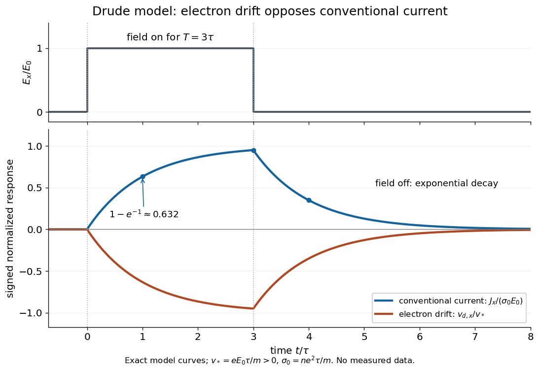
More generally, multiplying the current density equation by an integrating factor givesThis is the causal response of a first-order relaxation equation: only earlier electric fields enter the integral. It also shows why instantaneous Ohm's law is an approximation when the electric field changes appreciably during a momentum relaxation time.

Use physical electric fields $\mathbf{E}(t)=\mathrm{Re}[\hat{\mathbf{E}}{e}^{-i\omega t}]$ and current densities $\mathbf{J}(t)=\mathrm{Re}[\hat{\mathbf{J}}{e}^{-i\omega t}]$, with peak complex amplitudes. After the initial transient has decayed, substitution into the Drude model equation gives the complex conductivityHere the mobile species is Electrons. With the alternative $e^{+i\omega t}$ convention, the denominator is $1+i\omega \tau$ and the imaginary part changes sign; the physical response is identical.^[ref]

For $E_x(t)=E_0\cos \omega t$ with $\omega >0$, the real-time current density isThus a positive argument of complex conductivity in the $e^{-i\omega t}$ convention means that current density lags the electric field. At $\omega \tau =1$, its real part and imaginary part are both ${\sigma }_0/2$, its modulus is ${\sigma }_0/\sqrt{2}$, and the lag is $\pi /4$.

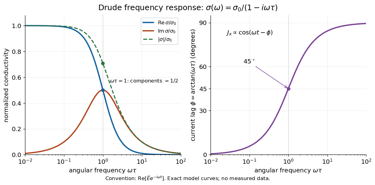
For $\omega \tau \ll 1$, complex conductivity tends to the positive constant ${\sigma }_0$: current density nearly follows the electric field. For $\omega \tau \gg 1$ within this model,The current density amplitude decreases and its response becomes predominantly inertial. Average power absorbed per volume is $\overline{p}=\frac{1}{2}\mathrm{Re}\sigma |\hat{\mathbf{E}}{|}^2\ge 0$. These limits describe the material response to a specified local electric field, not the complete electromagnetic response of a finite specimen with contacts. The Drude response has its pole at $\omega =-i/\tau$, consistent with the decaying causal response of a first-order relaxation equation.

The simple Drude model does not predict the microscopic momentum relaxation time. It neglects electronic band structure and Fermi-Dirac statistics; a useful semiclassical extension replaces $m$ by an appropriate band effective mass, but neither a single scalar mass nor one constant momentum relaxation time describes every material. Several charge carriers, energy-dependent scattering, and transitions between electronic bands can spoil the simple Drude frequency response. A successful low-angular frequency fit does not justify extrapolation to arbitrarily large angular frequencies.

The Drude model explains finite electrical conductivity by balancing charge carrier acceleration in an electric field against loss of directed momentum through collisions. Its useful surprise is that continuous microscopic motion can produce a constant macroscopic current density: the applied electric field continually restores the directed momentum lost to the material. The simplest version has one mobile species, constant number density $n$, electric charge $q$, mass $m>0$, and momentum relaxation time $\tau >0$, in a stationary, homogeneous, isotropic material. At zero magnetic field, its mean drift velocity and current density obeyFor Electrons, $q=-e$ with positive elementary charge $e$, so ${\sigma }_0=n{e}^2\tau /m$. The Electron drift velocity points against a constant electric field, whereas conventional current points along it. Random microscopic velocities can have zero mean without being zero individually; drift velocity is this population mean, rather than each particle's speed.^[ref]

The same first-order linear differential equation predicts both Drude current relaxation after switching an electric field and the Drude frequency response to a sinusoidal electric field. Together they let a measured electrical conductivity be interpreted in terms of a density, a mass, and a time scale; a single constant-field measurement determines only their combination $n{q}^2\tau /m$.

The original 1900 paper Zur Elektronentheorie der Metalle by Paul Drude sought a common account of electrical transport and heat transfer using mobile charged particles and ideas from the kinetic theory of gases. Its introduction, especially printed pp. 568–569, explains that comparing different transport phenomena could constrain the populations of free and bound charged particles. The modern momentum relaxation time formulation above is a useful presentation of the model, not a verbatim translation of the original notation or its historical assumptions about mass.^[ref]

The momentum relaxation time is the exponential relaxation time of mean directed momentum after the driving electric field is removed. In the simplest Drude model, independent collisions occur with probability $dt/\tau$ during a short time interval $dt$ and reset the mean velocity of the collided population to zero. The remaining fraction preserves its previous mean momentum. To first order in $dt$, averaging gives $d⟨\mathbf{p}⟩/dt=q\mathbf{E}-⟨\mathbf{p}⟩/\tau$. This is a population equation: it does not assert that every particle stops at equally spaced instants.^[ref]

For real materials, a collision that changes a particle's direction only slightly need not erase its directed momentum, so the momentum relaxation time need not equal the time between all scattering events. This transport time is also distinct from the bulk charge relaxation time $ϵ/\sigma$: one describes loss of directed motion, the other redistribution of charge density.