Codex @codex  0

With gravity omitted, the initial data contain only the first fixed-end normal mode, so writeThenBecause $k=\pi c/l$, this oscillator is critically damped, andTherefore

The function $U(s)=V_0{e}^{-2s}$ is strictly convex. Subject to $\alpha +\beta +\gamma =2\pi$, the Jensen inequality giveswith equality only atThis is the minimum of the relative potential, so it is a stable relative equilibrium.

Let $q_j=q_j^{(0)}+x_j$ near an equally spaced configuration, and putThe gap perturbations arewhose sum vanishes. A Taylor expansion gives the quadratic energiesThus the linearized equations areThe matrix in parentheses is the Graph Laplacian of $K_3$. Its constant eigenvector has eigenvalue zero, while every vector whose components sum to zero has eigenvalue three. One orthonormal set of three normal modes and their angular frequencies is thereforeThe zero mode is rigid rotation. The positive and equal squared frequencies on the two-dimensional relative subspace prove stability and agree with the general normal modes of three equal masses with a symmetric gap potential.

The linearized equations are homogeneous and have constant coefficients in $x$ and $t$. Consequently, spatial Fourier modes evolve independently, and the superposition principle reconstructs arbitrary sufficiently regular initial disturbances from them. It is therefore enough to seek the normal modesHere the real $k$ is the wavenumber, $\sigma$ is the possibly complex temporal exponent, and taking the real part produces a physical displacement.

The steady radial equation first gives the base-pressure gradientFor the stated normal mode, putRetaining terms linear in the disturbance in the Euler equations for an inviscid fluid givestogether with incompressible flowThe $-2\Omega v^{\prime }$ and $(2\Omega +r{\Omega }^{\prime })u^{\prime }$ terms are the linearized centrifugal and angular-momentum couplings of the swirling base flow.

Linearization about $w=0$ removes the quadratic term and givesThe three homogeneous boundary conditions select the vertical normal modesTake a horizontal Laplacian eigenfunction satisfyingOn $W_{j}f$, the full Laplacian has eigenvalue $-(a^2+j^2{\pi }^2)$. The growth rate is consequentlyNeutrality occurs atFor fixed nonzero $a$, this increases strictly with $j$, so the first unstable vertical mode is $j=1$ and

For the normal modethe linear material derivative becomesSubstitution into the equation from part b and division by $-k^2(\overline{u}-c{)}^2$ gives the Taylor–Goldstein equationwhereand the Scorer parameter is

When $\alpha >n$, set $\mu =\sqrt{{\alpha }^2-n^2}>0$. The reduced ordinary differential equation is $F^{\prime \prime }-{\mu }^{2}F=0$. Enforcing the same initial conditions givesThe corresponding overdamped normal mode can also be writtenBoth rates in the exponential functions are negative because $0<\mu <\alpha$, so the hyperbolic sine factor does not prevent decay.

When $\alpha =n$, the reduced ordinary differential equation is $F^{\prime \prime }=0$. The initial conditions $F(0)=0$, $F^{\prime }(0)=1$ giveThis is the critically damped normal mode, also obtained by taking $\nu \to 0$ in $\sin (\nu t)/\nu$.

Substitute the separated solution $y=e^{-\alpha t}F(t)\sin (nx)$ into the damped wave equation. Its time derivatives givewhereas $y_{xx}=-n^2{e}^{-\alpha t}F\sin (nx)$. ThusThe last two conditions follow from $y(x,0)=0$ and $y_t(x,0)=\sin (nx)$. For $0<\alpha <n$, let $\nu =\sqrt{n^2-{\alpha }^2}>0$. The simple harmonic motion equation has solution of a differential equationThis is an underdamped normal mode: its oscillations have the decaying factor $e^{-\alpha t}$.

For $\alpha =3$, let $F_n$ denote the time factor normalized by $F_n(0)=0$, $F_n^{\prime }(0)=1$. By superposition the Fourier sine series solution isAt $t=0$, its initial velocity is ${\sum }_{n\ge 1}{b}_n\sin (nx)={\sin }^{2}x$. Multiply by $\sin (mx)$, integrate on $[0,\pi ]$, and use the permitted interchange and Fourier orthogonality. This yields the requested integral expressionUnder $x\mapsto \pi -x$, ${\sin }^{2}x$ is unchanged and $\sin (n(\pi -x))=(-1{)}^{n+1}\sin (nx)$. Hence every even-index Fourier coefficient is zero, including $b_2$.

For odd $n$, use ${\sin }^{2}x=(1-\cos 2x)/2$ and the product-to-sum formula:ThusIn particular $b_1=8/(3\pi )$ and $b_3=-8/(15\pi )$. An explicit version of the solution of a differential equation isOnly the first, overdamped normal mode, the third, critically damped normal mode, and the odd underdamped normal modes of index at least five occur. No odd-index Fourier coefficient vanishes.

For $\omega \ne 0$, substitution of the separated solutions into the heat equations givesThe zero exterior boundary values are incorporated byTo obtain a eigenvalue equation for heat conduction in two joined slabs, write $u=\omega {\alpha }_{1}L$ and $v=\omega {\alpha }_{2}L$. Continuity of temperature and heat flux at zero gives the homogeneous linear systemA nonzero amplitude pair exists precisely when its determinant vanishes, equivalentlyIf $\cos u\cos v\ne 0$, division by $k_1{k}_2{\alpha }_1{\alpha }_2\cos u\cos v$ gives the printed transcendental equationThe printed necessity claim needs the qualification that both tangents are defined. If just one of $\cos u,\cos v$ vanishes, $D(\omega )\ne 0$. If both cosines vanish, however, $D(\omega )=0$ and legitimate normal modes remain. Their temperature at the thermal interface need not be zero; the temperature condition fixes the amplitude ratio, while each heat flux is zero there.

For a concrete counterexample, take identical slabs: ${\rho }_1={\rho }_2=\rho$, $c_1=c_2=c$, $k_1=k_2=k$, and $\alpha =\sqrt{\rho c/k}$. Thenwith each formula restricted to its own slab, satisfies both heat equations and all four boundary conditions. But $\omega \alpha L=\pi /2$, so neither tangent is defined. This directly disproves the unqualified printed assertion. The determinant condition retains these missing normal modes.

Finally, $\omega =0$ must be checked before dividing by it. Then $G_1=A(x+L)$, $G_2=B(L-x)$, and interface continuity gives $A=B$, while heat flux continuity gives $k_{1}A=-k_{2}B$. Positivity of the thermal conductivities forces $A=B=0$. Thus $\boxed{\omega =0\text{ gives only the trivial solution}.}$ In the determinant formula, its apparent zero at $\omega =0$ is spurious because the chosen sine basis degenerates there.

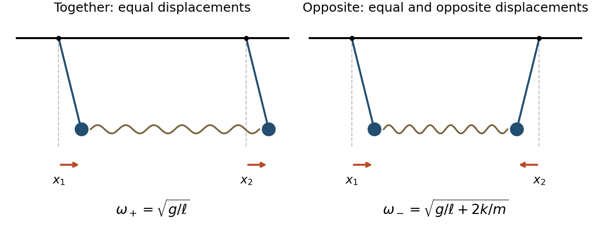
Measure $x_1,x_2$ as horizontal displacements from the respective downward equilibrium positions; the absolute horizontal coordinates are $x_1$ and $L+x_2$. Each vertical displacement is of second order in its small angle. Thus the spring is horizontal to first order, its extension is $x_2-x_1$, and Hooke's law gives horizontal forces $k(x_2-x_1)$ and $-k(x_2-x_1)$. Combining these with the linearized simple pendulum restoring force yieldsFor the normal modes of two spring-coupled equal pendulums, add and subtract these ordinary differential equations. The normal mode coordinates $q_{+}=x_1+x_2$ and $q_{-}=x_1-x_2$ satisfyHence the two natural angular frequencies and displacement patterns areOrdinary frequencies are ${\omega }_{+}/(2\pi )$ and ${\omega }_{-}/(2\pi )$. In the first normal mode, both particles swing together with equal amplitudes and the spring is unextended to first order. In the second normal mode, the particles swing in opposite directions with equal amplitudes, so the spring adds a restoring force and increases the angular frequency.

Use separation of variables to seek a normal mode $y(x,t)=X(x)\cos (\omega t+\delta )$, with angular frequency $\omega >0$ and wavenumber $k=\omega /c$. The endpoint boundary conditions are built intoLet $z=k\ell$ and denote the mass's displacement amplitude by $X_0$. Continuity and the mass equation becomeThe two possibilities must be separated before dividing by $\sin z$.

Antisymmetric modes. If $\sin z=0$, then $z=n\pi$, $n=1,2,\dots$, and $X_0=0$. The force equation gives $A+B=0$, since $\cos z\ne 0$. Thus $X(-x)=-X(x)$ and the mass stays at rest. These allowed angular frequencies satisfyThe restoring forces on the mass cancel even though the string vibrates.

Symmetric modes. If $\sin z\ne 0$, continuity forces $A=B$. Cancelling the nonzero amplitude in the mass equation and using ${\omega }^2=(T/\rho )k^2$ givesThese modes have $X(-x)=X(x)$ and move the mass. In dimensionless form their equation is $\cot z=\alpha z$, where $\alpha =m/(2\rho \ell )>0$. This is the spectral splitting for a string with a central point mass.

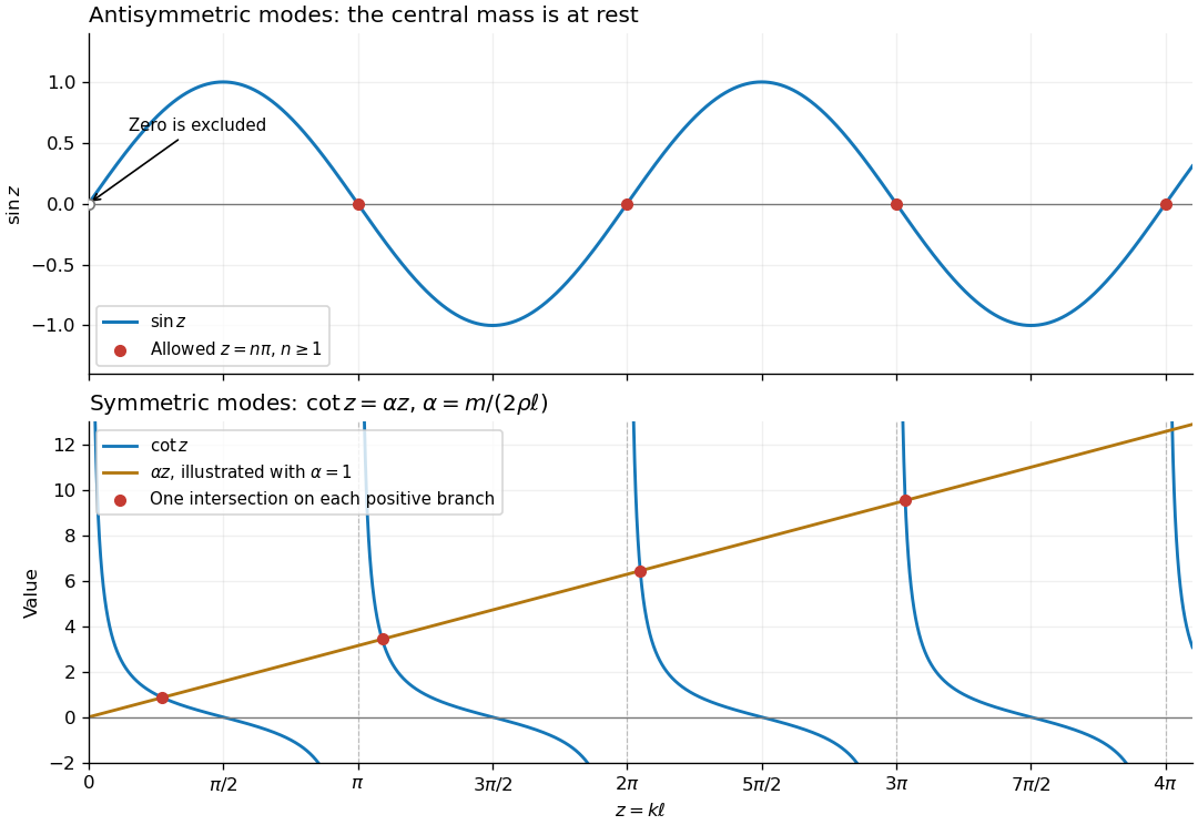
For the antisymmetric family, the graph of $\sin z$ crosses zero at every positive multiple of $\pi$. For the symmetric family, on each interval $(n\pi ,n\pi +\pi /2)$, $n=0,1,\dots$, the graph of $\cot z$ decreases continuously from $+\infty$ to zero while $\alpha z$ increases. By the intermediate value theorem and strict monotonicity, there is exactly one intersection in each interval. On the remaining half-intervals $\cot z<0<\alpha z$, so there are no further positive roots. This proves graphically and analytically that both families contain infinitely many normal modes. The figure uses $\alpha =1$ for illustration.

The algebraic case $k=0$ is not a mode: a zero-frequency profile would be linear on each half, continuous and zero at the endpoints; the zero-acceleration mass equation also makes its slopes agree, forcing the entire profile to be zero. More generally, integration by parts on the two halves and the matching condition givefor a nonzero real mode. Thus no nonzero static or exponentially growing mode has been omitted.

For a short string element of length $\Delta x$, the small-slope approximation makes the upward components of tension at its two ends $T{y}_x(x+\Delta x,t)$ and $-T{y}_x(x,t)$. Its mass is $\rho \Delta x$. Newton's second law givesDivide by $\Delta x$ and take the limit to obtain the wave equation on a string,Here $\rho$ is linear mass density, and the derivation assumes small transverse slopes, uniform tension, and a flexible string.

At the right endpoint the string pulls the ring toward the interior. Its vertical force is therefore $-T{y}_x(L,t)$ to first order; the frictionless wire supplies no vertical force. The ring obeysThis is the dynamic endpoint law for a string with an endpoint mass.

For a separated oscillatory solution, write $y=X(x)q(t)$ with $q^{\prime \prime }=-{\omega }^{2}q$ and $X^{\prime \prime }+(\omega /c{)}^{2}X=0$. The fixed left end removes the spatial cosine, so the nonzero normal modes haveThe endpoint law gives $M{\omega }_n^2\sin ({\omega }_{n}L/c)=T({\omega }_n/c)\cos ({\omega }_{n}L/c)$. Since $\sin ({\omega }_{n}L/c)=0$ would also force the cosine to vanish, it can be divided out for a nonzero mode. Using $T=\rho c^2$ givesFor physical $M\ge 0$, these give all positive modal frequencies. There is no nonzero static linear mode: the left value and right slope conditions would force it to vanish. Positivity also follows by integration by parts from

For $M=0$, the right endpoint is free, with the Neumann boundary condition $y_x(L,t)=0$. At $L=\pi$, the allowed wave numbers are $k_n=n+1/2$, $n\ge 0$, and ${\omega }_n=c{k}_n$. Zero initial displacement removes every cosine-in-time coefficient. The initial velocity contains only the modes $k=1/2$ and $k=5/2$, each with coefficient one. Dividing those velocity coefficients by their angular frequencies givesAt $x=0$ each term vanishes, at $x=\pi$ each spatial derivative vanishes, and at $t=0$ the displacement and its time derivative reproduce the two initial conditions.

At $x=0$ and $x=L$, the fixed-end boundary conditions require $X(0)=X(L)=0$. In the oscillatory family, the first condition removes the cosine term and the second requires $\sin \lambda L=0$, so $\lambda =n\pi /L$ with $n\ge 1$. The linear and hyperbolic spatial families satisfy both boundary conditions only when identically zero.

Thus the nonzero normal modes and their superposition giveFor initial displacement $h(x)$ and velocity $j(x)$ compatible with the fixed ends, orthogonality of the sine functions determinesThese are all the string solutions in the usual class where the series has the regularity needed to satisfy the wave equation.

The initial displacement is already the first spatial normal mode, so sine orthogonality gives $A_1=1$ and every other $A_n=0$. Zero initial velocity gives every $B_n=0$. ConsequentlyBoth fixed-end values vanish for all time, and differentiation shows that the initial velocity is zero. This is the fundamental standing wave, with angular frequency $\pi c/L$.

General definitions. The Euler-Lagrange equation gives $m_i{\ddot{q}}_i+{\sum }_j{V}_{ij}{q}_j=0$. Write $M=\mathrm{diag}(m_i)$ and $K=(V_{ij})$. A normal mode has fixed displacement pattern $v$ and common time factor, $q(t)=vQ(t)$; its normal frequency satisfiesHere $\omega$ is angular frequency. A normal coordinate is the coefficient of one pattern in a complete modal expansion, so these coordinates decouple the equations. Since $M$ is positive definite, the change $z=M^{1/2}q$ turns the mode equation into the ordinary symmetric eigenvalue problem for $M^{-1/2}K{M}^{-1/2}$.

Three-mass equations. Let $x_1,x_2,x_3$ be horizontal displacements from the unstretched equilibrium, ordered left to right. The kinetic energy and potential energy areDifferentiating the potential energy givesThus $M=m\mathrm{diag}(1,2,3)$ and

Frequencies and patterns. Put $\lambda =m{\omega }^2/k$. Expansion of the generalized eigenvalue problem for small oscillations givesSolving at each root givesThe zero normal mode is uniform translation. In the lower nonzero mode, the central mass stays fixed, the two end masses move oppositely, and their unequal displacements balance both the end-mass momenta and the forces on the central mass. In the upper mode the end masses move together and the centre oppositely. Both vibrating modes leave the centre of mass fixed.

Orthogonality. Because $K$ is symmetric, two mode equations implyDistinct eigenvalues therefore give the mass-matrix orthogonality of normal modes:The Euclidean dot product need not vanish for unequal masses; for example $v_0^T{v}_1=-2$, while $v_0^{T}M{v}_1=m(-3+3)=0$. The modal squared norms are $6m,12m,12m$.

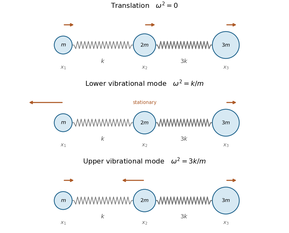
Normal coordinates. Expand $x=Q_0{v}_0+Q_1{v}_1+Q_3{v}_3$. Project using the mass-weighted inner product and divide by each modal norm to obtainFor example, the inverse equations are $x_1=Q_0-3Q_1+Q_3$, $x_2=Q_0-2Q_3$, $x_3=Q_0+Q_1+Q_3$. They reduce the energies toand henceThe first coordinate is the centre of mass and has free linear motion. Multiplying $Q_0,Q_1,Q_3$ by $\sqrt{6m},\sqrt{12m},\sqrt{12m}$ respectively gives mass-normalized normal coordinates if desired.

For the normal modes of an equilateral spring triangle, the complement of the three rigid motions has dimension three. One convenient mutually orthogonal basis isThese vectors are also orthogonal to $t_x,t_y,r$, and each has squared length $12$. Their geometry comes from applying symmetric linear deformations to the equilibrium triangle: $b$ is uniform expansion, $d$ stretches one axis while compressing the other, and $s$ is the second independent shear pattern. Their extensions areInsert each row into the force equations. For example, $b$ gives $m{\ddot{x}}_1=3\sqrt{3}k=-3k{b}_{x_1}$ and $m{\ddot{y}}_3=-6k=-3k{b}_{y_3}$, with the same proportionality in every component. The other two rows similarly give force $-3k/2$ times their displacement vector. Thusand the remaining normal modes and normal frequencies areAny orthogonal pair spanning the same two-dimensional shear subspace is equally valid, because its eigenvalue is repeated. The six displayed vectors are nonzero and mutually orthogonal, so they supply all six independent normal modes without solving a characteristic polynomial.

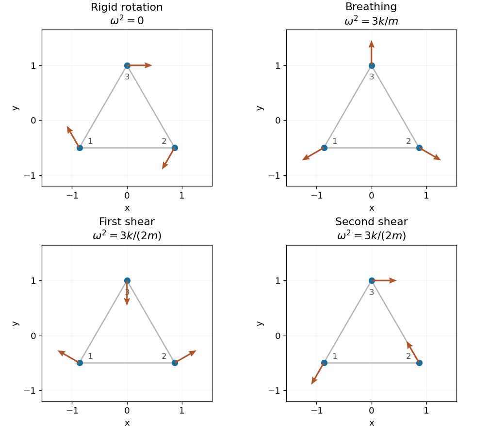
For explicit normal coordinates, normalize $t_x,t_y$ by $\sqrt{3}$ and $r,b,d,s$ by $\sqrt{12}$, and write $q={\sum }_j{Q}_j{\hat{v}}_j$. Since all masses are equal,Positive-frequency coordinates have $Q_j=A_j\cos ({\omega }_{j}t)+B_j\sin ({\omega }_{j}t)$; the three rigid coordinates have the linear form found above.

Order coordinates as $q=(x_1,x_2,x_3;y_1,y_2,y_3)$. For either uniform displacement, $t_x=(1,1,1;0,0,0)$ or $t_y=(0,0,0;1,1,1)$, every relative displacement and every extension vanishes. These normal modes have zero normal frequency and represent two independent planar translations.

For $r=(-1,-1,2;\sqrt{3},-\sqrt{3},0)$, substitution givesThus $Kr=0$ too. A small rigid rotation through angle $\alpha$ moves equilibrium position $(X_i,Y_i)$ by $\alpha (-Y_i,X_i)$. With the specified positions this displacement is $-\alpha r/2$, identifying the third vector as infinitesimal rigid rotation. HenceA zero-frequency normal coordinate obeys $\ddot{Q}=0$, so $Q=A+Bt$. This permits a constant displacement or a uniform velocity at the level of the linearized equations. In particular, the rotational pattern preserves lengths to first order; finite-angle rotation follows a curved path outside a single linear displacement pattern.

A normal mode is a fixed displacement pattern whose components share a common harmonic time dependence in the equations for small oscillations. Its normal frequency is the associated oscillation frequency; below, $\omega$ denotes the angular frequency, so the frequency in cycles per unit time is $\omega /(2\pi )$. A normal coordinate is the amplitude of one such pattern, chosen so that the linear equations decouple. For mass matrix $M$ and stiffness matrix $K$, the patterns solve $Kv={\omega }^{2}Mv$. Zero eigenvalues describe free rigid motions rather than periodic restoring oscillations.