Using mass for the dominant lithium isotope gives a transition wavenumber . Inserting the thermal speed into the stated Doppler broadening expression givesThe supplied formula is the Gaussian half width at half maximum; the corresponding full width is about . Meanwhile exponential population decay with lifetime produces a natural linewidth expressed as a full widthHere must be in in the second expression. Equivalently the fine-structure separation is about GHz, the Doppler half width about GHz, and the natural linewidth expressed as a full width about MHz. The natural linewidth is therefore negligible compared with thermal broadening; low density also makes collision broadening less important.
The doublet is resolvable in principle, but only marginally against the Doppler width. The separation exceeds one Doppler full width, so two components can survive, although their profiles overlap strongly. The and upper levels have different statistical weights, so the weaker member need not make an equally conspicuous maximum. A spectral resolving power is the basic instrumental requirement; a width well below and adequate signal would make the test more convincing. An arbitrarily fine spectrometer cannot remove the physical Doppler overlap. This conclusion uses the stipulated thermal, optically thin picture; additional photospheric velocity fields or optical-depth effects would require more information.
Use the D3h molecular point group for phosphorus pentafluoride, with along the two axial P–F bonds. For each symmetry operation, only atoms left in place contribute to the character of the Cartesian displacement representation; each contributes the trace of the corresponding spatial matrix. In the class order this givesFor example a fixes P and one equatorial F, and each fixed atom has Cartesian trace , giving . reflection in the equatorial plane fixes four atoms, each with trace , giving . Reduction with the character table givesSubtract translations and rotations to obtainIts dimension is , as required for a nonlinear six-atom molecule. Thus there are eight symmetry-distinct fundamental frequencies in the harmonic picture, with each E mode doubly degenerate. This analysis concerns vibrations about one trigonal-bipyramidal minimum; it does not treat large-amplitude rearrangements between minima.
The octahedral splitting separates the metal and orbital sets. The Racah parameter characterizes interelectronic repulsion and hence the spacing of many-electron d-shell terms; it is not another name for . A Tanabe-Sugano diagram plots term excitation energies against , for specified values of the other repulsion-parameter ratios. Each ordinate is measured relative to whichever term is the ground state at that field strength. The original many-electron treatment diagonalizes the relevant d-shell energy matrices rather than identifying every absorption with a one-electron gap.[ref]
On the Absorption Spectra of Complex Ions. I by Yukito Tanabe and Satoru Sugano. 1954, pp. 753–766, d-shell energy matrices in a cubic field
The ground state changes from high-spin , , to low-spin , . The larger splitting eventually compensates the additional pairing cost. Because all plotted excitation energies are re-referenced to the new ground state, the branches change slope at the crossover. The break is not an infinite physical excitation energy or a discontinuity of the underlying Hamiltonian.
Here , so the ground term is . There are no spin-allowed d–d bands in the displayed manifold under the spin selection rule: the excited terms shown have doublet or quartet rather than sextet multiplicity. Very weak spin-forbidden absorptions can still gain intensity through spin–orbit coupling, and even spin-allowed d–d transitions would be forbidden by the Laporte rule in ideal centrosymmetric coordination. Thus a strong ordinary d–d spectrum should not be predicted simply by multiplying the splitting by a numerical factor. For scale, the lowest quartet branches read roughly at this abscissa, corresponding to weak features around , and if such forbidden intensity is detectable. These are graphical estimates, not precision assignments of every weak line.
Now and the ground term is . Spin-conserving transitions to the labelled doublet excited terms are possible. Reading the diagram gives approximatelyThe first two upper terms are coincident or unresolved at this diagram's resolution. These doublet transitions should dominate over the spin-forbidden transitions to sextet or quartet levels. Their intensity still depends on vibronic or other relaxation of the Laporte rule. The plotted curves justify only approximate wavenumbers, not several-digit band positions.
Let and treat the quencher concentration as a constant reservoir. Weak steady excitation, one emitting population, and the three specified processes giveDividing the fluorescence photon-production rate by the absorbed photon rate therefore givesThis assumes no saturation, photochemical loss, reabsorption, static association or additional excited-state decay, and that each counted absorbed photon reaches the stated population. In this restricted scheme and the unquenched lifetime is .
Rearrangement gives the Stern-Volmer equationThus a straight-line plot against has unit intercept and slope . Determine using an independently measured unquenched lifetime, or use known in the restricted model. Yield measurements alone do not separate two unknown rate constants. Equivalently the slope of is .
Use the absorbed intensity rather than incident intensity to normalize samples, and correct solvent/background signals, quencher absorption and fluorescence reabsorption. Under dynamic fluorescence quenching the lifetime ratio should follow the same straight line as the yield ratio. A reduced intensity without the corresponding lifetime change suggests static fluorescence quenching or an optical artefact; curvature can also indicate multiple populations or more complicated kinetics.
A quencher-independent intersystem-crossing rate adds to the unquenched decay rate:The normalized Stern-Volmer equation retains the same form, so intersystem crossing does not bias if the actual unquenched lifetime is used. It reduces below one and changes the slope through ; assuming would then give the wrong result. A quencher that itself changes intersystem crossing or returns triplet population to the singlet requires a larger kinetic scheme.
Writing and , the normalized determinant isIts two spin orbitals are orthogonal because , even if the spatial atomic functions have nonzero overlap. Exchanging both the spatial and spin coordinates of the two electrons reverses the sign, as required for fermionic antisymmetry.
At this separation the orbital overlap and interatomic two-electron exchange integrals are negligible. Each localized electron then contributes essentially the isolated hydrogen energy, while the interatomic electrostatic terms cancel to leading order for neutral fragments. Including nuclear repulsion in the molecular energy givesThe closed-shell RHF determinant instead doubly occupies . It retains ionic configurations with both electrons on the same atom, even at dissociation. Using atomic units and the Hartree energy in the stated unrelaxed hydrogenic 1s basis, the same-atom two-electron Coulomb integral is . Consequently at infinite separationwhere energies and integrals inside the first expression are in atomic units. It is much too high compared with two neutral atoms. Retaining the leading intersite Coulomb term at gives , still about above UHF. The numerical RHF estimates specify the supplied fixed 1s basis; a larger optimized orbital space changes them. If nuclear repulsion is excluded by an electronic-energy convention, subtract the same from both quoted total molecular energies. The restricted/unrestricted comparison and their dissociation behaviour are unchanged.[ref]
XXXIV. Notes on the molecular orbital treatment of the hydrogen molecule by Charles Alfred Coulson and Inga Fischer-Hjalmars. 1949, pp. 386–393, minimal atomic-1s molecular-orbital treatment
The fixed localized determinant is unsuitable near equilibrium. It does not develop the correct shared bonding orbital and is not a pure singlet: for one alpha and one beta orbital, , which is nonzero unless the occupied spatial orbitals coincide. At dissociation it is an equal singlet/triplet mixture, though their energies become degenerate there. Near equilibrium the physical ground state is a bonding singlet. An optimized UHF calculation can recover the restricted, spin-pure solution by making its two occupied spatial orbitals equal; that does not rescue the particular fixed atomic-orbital determinant written here. A spin-adapted multideterminant description is needed to combine good bonding near equilibrium with correct singlet dissociation.
Number the four sites of the cyclobutadienyl dianion cyclically and apply the Hückel method. The orthonormal pi basis givesA convenient real orthonormal eigenbasis isThus one bonding and two degenerate nonbonding orbitals are filled, and the antibonding orbital is empty. There are six pi electrons, including the two added by the dianion charge. Rotating the two occupied nonbonding orbitals within their degenerate subspace changes their individual sketches but not the total density matrix.
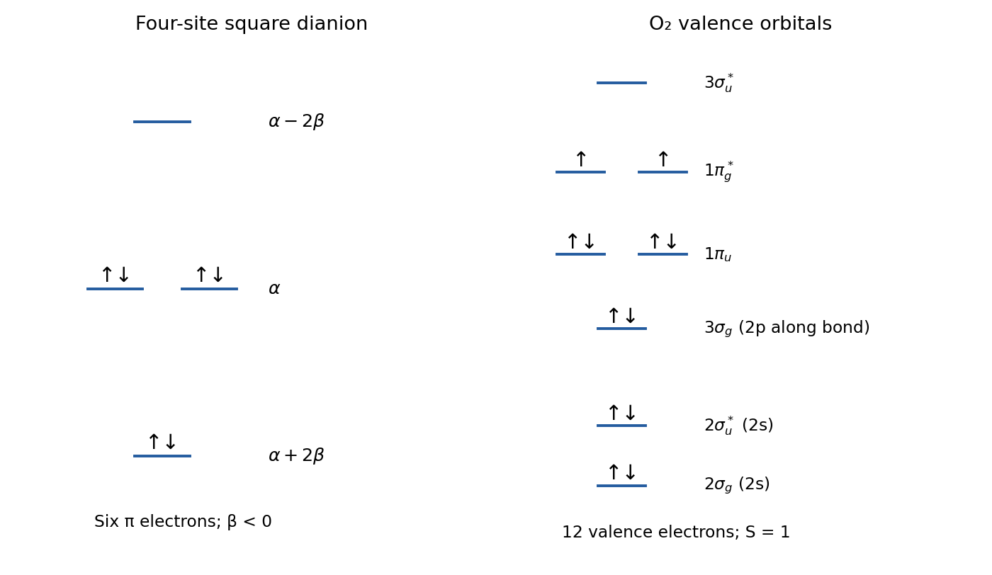
Original orbital levels and occupations for the four-site dianion and valence O2
. Details. The Hückel orbital charge density and Hückel pi bond order giveEach site receives electron from the lowest orbital and one from the occupied nonbonding subspace, so at every carbon, summing to six. Relative to one neutral pi electron per carbon this is a pi charge of at each site.
For adjacent sites, only the lowest orbital contributes, giving . For opposite sites the nonbonding contribution reverses the sign: . These non-neighbour negative density-matrix entries are not extra sigma bonds or extra resonance integrals in the Hamiltonian. If only skeletal nearest-neighbour pi bond orders are requested, the four values are the relevant ones.
configuration interaction with singles and doubles (CISD) uses a linear combination of the reference Slater determinant and singly and doubly excited determinants. Its many-electron trial state is therefore not restricted to one determinant; the orbitals may be held fixed while the configuration coefficients are varied.
Kohn-Sham equations in density functional theory use an auxiliary one-electron Hamiltonian whose effective potential depends on the density. Its orbitals construct a density representing an interacting electronic system; this is distinct from explicitly diagonalizing a large many-electron determinant Hamiltonian.[ref]
Self-Consistent Equations Including Exchange and Correlation Effects by Walter Kohn and Lu Jeu Sham. 1965, pp. A1133–A1135, ground-state effective one-electron formulation
molecular mechanics evaluates a parametrized potential of atomic positions, with terms such as bond stretching, angle bending, torsion and nonbonded interactions. electrons are represented implicitly through the fitted force field, rather than by electronic orbitals, a density or an electronic wavefunction. This example is different from both preceding electronic methods.
For conventional CISD, the leading matrix-vector contraction scales as in occupied and virtual orbital dimensions. If both grow proportionally to a system-size parameter , the familiar estimate is work per iteration; the iteration count and integral-storage strategy add implementation-dependent costs.
Calculated potential energy surfaces can predict equilibrium geometries and harmonic force constants, permitting comparison with diffraction-derived structures, rotational constants and vibrational spectra. Calculating several roots or different charge states can also estimate excitation or ionization energies. Such predictions depend on basis and truncation quality; truncated CI is not generally size extensive and is not automatically reliable for strongly multiconfigurational bond breaking. The quoted polynomial scaling is for CISD, not full configuration interaction, whose determinant space grows combinatorially.
An alternant hydrocarbon has a pi-site graph that can be divided into two sets so that every retained neighbouring resonance interaction joins different sets. Equivalently, the graph is bipartite. A chain and an even ring satisfy this condition; an odd ring does not. The classification refers to the model's coupling graph, rather than simply to which bonds are drawn double in one Lewis structure.
Write with the same carbon diagonal parameter throughout, and define to have entries on one sublattice and on the other. Bipartite connectivity impliesThus implies . This proves energy pairing about , , and equal site-probability magnitudes in each paired pair, since . This is the Coulson-Rushbrooke pairing property.[ref]
Note on the method of molecular orbitals by Charles Alfred Coulson and G. S. Rushbrooke. 1940, pp. 193–200, alternant-system pairing and density properties
For the usual neutral half-filled closed-shell occupation, the lower member of each pair is doubly occupied. Combining paired coefficients with completeness of the orthonormal basis gives one pi electron per carbon, so the model predicts no net pi charge separation. The same argument makes off-diagonal pi bond orders between sites on the same sublattice zero. These statements assume a neutral half-filled density and do not apply unchanged to the charged six-electron four-site ion considered separately.
An imbalance of sublattice sizes also guarantees at least nonbonding orbitals at energy , because the rectangular coupling block has insufficient rank to remove all its null space. None of the spectral pairing, equal paired densities, neutral charge uniformity or sublattice bond-order restrictions is required for a non-alternant graph. Long-range same-sublattice couplings or unequal diagonal parameters can likewise destroy the simple proof.
The coarse spacing is about , so . The two groups near 1.5 and therefore have and , respectively. For positive , increasing moves a component to lower wavenumber. The assignments areWithin one group, successive separations scale as . The observed gaps follow that pattern to their printed precision. There are distinct components because in the lower state; the and members remain coincident without an applied field. A high-resolution feature here is therefore not simply assigned to an arbitrary magnetic sublevel.
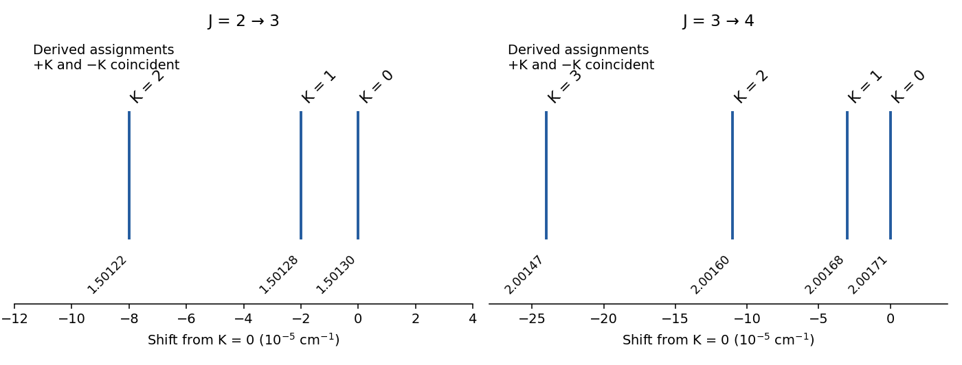
The lines give two equations independent of :Solving yields and . The small distortion is obtained by subtracting close numbers, so its precision is considerably worse than that of .
For components in a fixed group,For example the displacement gives , while gives . Both give ; the smaller gaps are consistent after rounding. The pure rotational transitions have , so the and terms cancel. Neither nor can be determined from these zero-field lines.
A spectral component shifts by the difference between its upper- and lower-level Stark shifts. With , and , the supplied energy formula givesFor radiation polarized parallel to the static field, , soThus the assigned feature has no first-order splitting, whereas the features acquire symmetrically arranged magnetic-sublevel components with spacings proportional to . With perpendicular radiation, gives the corresponding different allowed pattern. Recording field-dependent spectra with specified polarization would test both the J values and the K sequence; using an individual level's shift alone would not predict the observed line positions. Higher-order shifts of the nominally unsplit feature are outside this first-order test.
The largest applied field givesFor parallel polarization, adjacent allowed M values in a component are separated byAlready at this is for and for . Both exceed the stated resolution, and larger gives larger first-order spacings. The spectrometer should resolve suitable Stark components, provided their physical linewidths and signal-to-noise permit it. This predicts resolvable splittings rather than incorrectly comparing the maximum level shift directly with instrumental resolution.
A regularly repeated set of sharp features is characteristic of the unresolved Q subbranches of a perpendicular rovibrational band. The transition dipole is perpendicular to the symmetry axis, giving ; for the Q branch . Holding the rotational constants fixed between vibrational states cancels the term, leavingMany J transitions therefore coincide within each K-changing Q subbranch in this approximation. The different K subbranches are separated byThe P and R branches have and , respectively. Their extra J-dependent terms spread many transitions across a broad background at modest resolution. A parallel band, with , would not generate this repeated Q-subbranch spacing under the stated assumptions.
The subbranch spacing gives , hence . Rotation about the C–I symmetry axis has momentC and I lie on this axis, so only the three hydrogens contribute to . If is the I–C–H angle, their perpendicular distances are . Taking integer hydrogen mass givesThe molecular arrangement selects the obtuse solution, so . The supplementary acute angle describes the opposite axial direction, not the bond angle to iodine. This is a rigid-geometry estimate based on an effective rotational constant and the stipulated bond length, rather than a precision equilibrium-structure measurement.
In the Condon approximation the intensity from to contains the Franck-Condon factorThe lower ground-state vibrational wavefunction is localized near its equilibrium bond length. If the two equilibrium lengths are similar, it overlaps strongly with the upper wavefunction, but its overlap with highly excited upper vibrational states is usually small or suffers oscillatory cancellation. If the equilibrium lengths differ enough that a vertical excitation reaches the outer portion of the upper well, high- transitions can be strong while the overlap is small. Thus the two ends of a long progression are not normally both intense. This is an overlap argument, not a ban on either set of transitions; anharmonicity, a varying electronic transition moment and unusual wavefunctions can modify the intensity envelope.
Write the upper Morse oscillator term values in wavenumber units asThe spacing is . A Birge-Sponer plot therefore falls linearly in this model and can be extrapolated to zero spacing. If its horizontal coordinate is , the plotted line is . Its area from to its zero givesEquivalently a plot against has intercept and triangle area ; subtracting recovers . These conventions distinguish dissociation from the potential minimum and from the lowest vibrational level.
Measured consecutive members fix a local slope and intercept, so unobserved members can be supplied by extrapolation under an explicit spacing law. The upper-state limit on the absorption scale is . A local high-v fit can likewise estimate the remaining energy above an observed member without knowing its absolute v index. Near dissociation a real potential need not remain Morse-like, so an extrapolated triangle has model uncertainty; missing lines must not be silently assumed consecutive.
Successive differences remove the unknown absolute origin and the unknown initial vibrational quantum number. The five spacings are , , , and . Plot them at relative mid-indices . A straight-line fit givesThe curve reaches zero spacing at . Since a quadratic Morse progression has a spacing equal to its derivative at the interval midpoint, integrating the fitted line from the first observed relative level to estimates the energy still needed to reach the continuous limit:Thus the appropriate graphical conclusion is , not a many-digit threshold. Directly fitting a quadratic to the six measured transition positions puts its vertex at about , which checks the arithmetic but not the physical extrapolation law. The slight variation of second differences shows that extrapolating a constant anharmonicity beyond the observed range is approximate. No assignment of the arbitrary index n to an absolute upper-state v is needed.
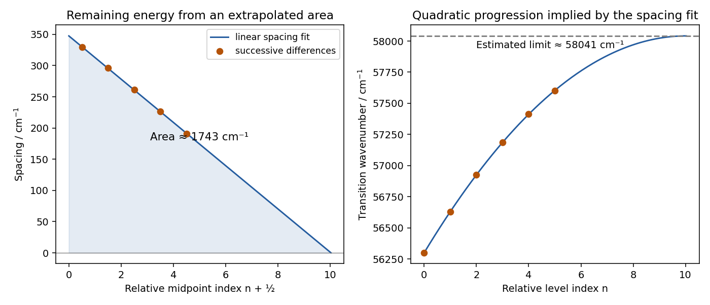
Original relative-index Birge–Sponer extrapolation and the inferred progression limit
. Details. Let . For a fixed row, moving one column to the right therefore givesThus adjacent-column entries decrease by the lower-state vibrational spacing, independent of the upper-state row in the ideal model. If the positive difference is instead defined as left minus right, it is . Stating the subtraction direction prevents an artificial negative vibrational frequency.
Averaging the left-minus-right differences across the three rows gives lower-state spacings of about and . Their difference is , soSimilarly, averaging successive down-column differences across the three columns gives upper-state spacings of about and . HenceUsing the first row and first column alone would give approximately and , respectively. The small inconsistency between nominally identical spacings is already present in the entries; it should be treated as limited data/model precision rather than fitted by assigning different lower-state constants to different rows. Values near for the lower state and for the upper state express the supported precision.
Choose x along O–O. The valence orbital order appropriate to O is approximatelyIts twelve valence electrons occupyThe two degenerate pi-antibonding orbitals are singly occupied with parallel spins according to Hund's rules. Thus , multiplicity , with three possible values. A triplet is a many-electron spin classification, not three electrons in one orbital. The resulting ground term is . Exchange stabilization favours this triplet over the singlets formed within the same frontier-orbital manifold.
Original valence-O2 diagram with the two singly occupied pi-antibonding orbitals
. Details. The active set contains four oxygen pi orbitals and two carbon pi orbitals, with eight electrons in six orbitals. The noninteracting levels, using the parameters inferred below, areEach bonding oxygen orbital has equal-phase coefficients on its two O atoms; its antibonding partner reverses one coefficient. The two pi directions are z in the prospective ring plane and y perpendicular to it. carbon pi and pi-star use z-directed p orbitals with equal and opposite coefficient signs. In this separated-fragment comparison the occupations are those of neutral triplet O plus neutral ethene. Do not refill the combined list solely by energy, which would move an electron between infinitely separated fragments and describe a charge-transfer state instead.
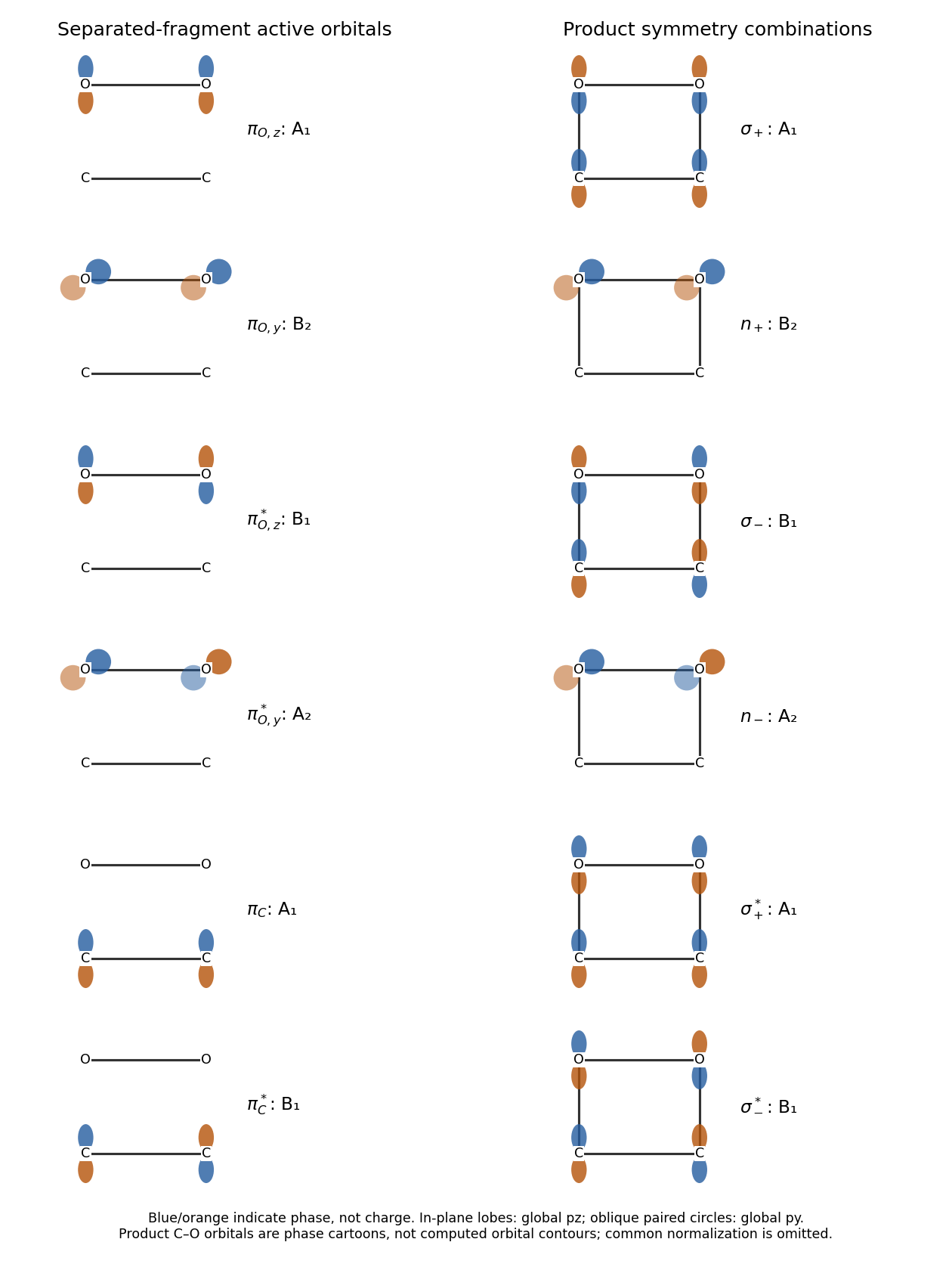
Original signed-orbital sketches for the six reactant and six product active orbitals
. Details. Use negative bonding Hückel resonance integrals, and . The oxygen HOMO is pi-antibonding, whereas the ethene HOMO is pi-bonding. The frozen-orbital Koopmans estimate therefore givesConsequently and . These Hückel Coulomb parameters are effective parameters of this spectroscopically calibrated model. Real ionization energies include relaxation and correlation, so they are not exact matrix elements of an isolated-atom Hamiltonian.
Let be localized bonding orbitals of the two new C–O bonds, and let be their antibonding partners. Their symmetry combinations areThe two remaining active orbitals are out-of-ring oxygen lone-pair combinations, . The opposite-phase combination is the HOMO in the supplied ordering and is HOMO−1. Both are filled, as are the two C–O bonding combinations, givingThe original active-orbital sketches show these phase relations, while the correlation diagram gives a qualitative energy ordering. Precise splittings between unrelated symmetry blocks are not determined by the fragment ionization energies. The retained O–O sigma bond, the C–C sigma bond and the other framework orbitals lie outside this six-orbital active comparison; the eight-electron count does not describe all valence electrons of the product.
The symmetric approach preserves the C2v molecular point group with its twofold axis z and mirror planes xz and yz. The molecular ring lies in xz. Classify orbitals by reflection signs : , , , . With globally defined p-orbital phases the molecular orbital correlation diagram givesWithin either two-orbital symmetry block the lower member remains correlated with the lower product member; the non-crossing rule prevents swapping their order through an ordinary same-symmetry crossing. Crossings between different irreducible representations are allowed. The crucial consequence is that the occupied carbon pi orbital correlates to a C–O-antibonding combination, rather than both initially occupied orbitals becoming the two product bonding orbitals.
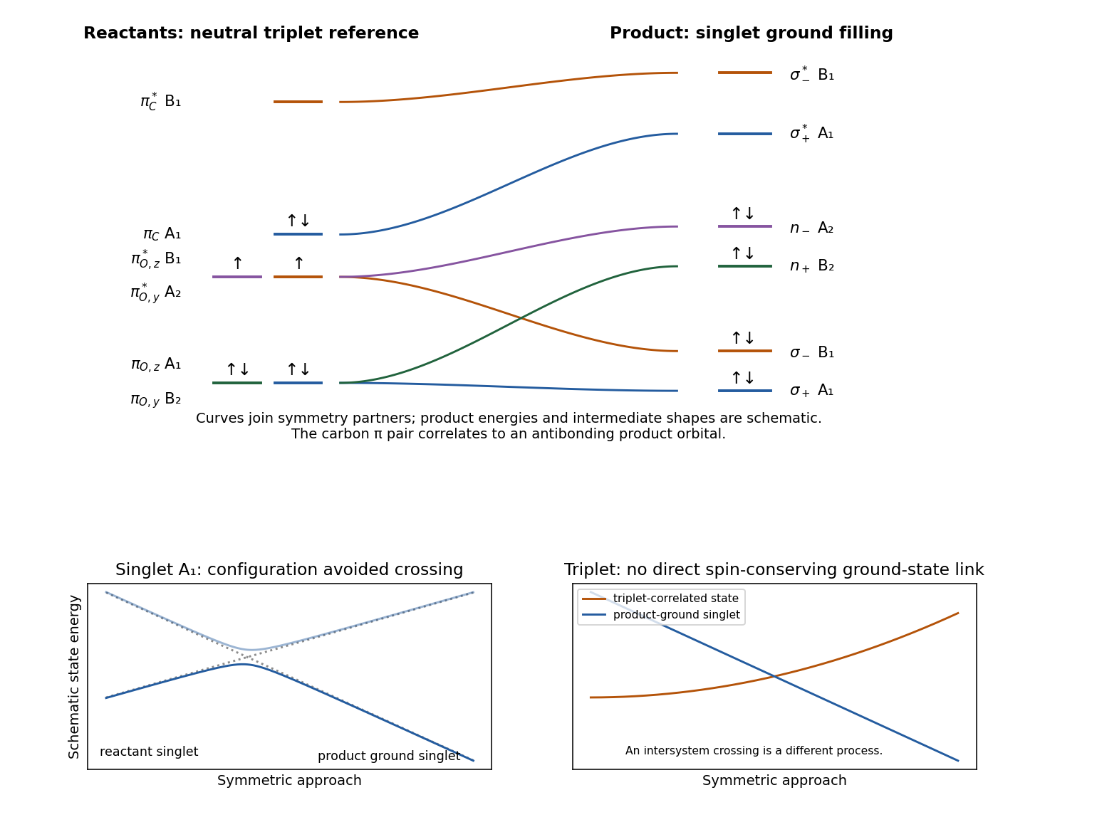


Endpoint energies, endpoint phase patterns and a conserved symmetry fix the qualitative connectivity. Each initial orbital must end in the appropriate product symmetry block, and the ordering within a generic block is preserved by avoided crossings. The two singleton blocks and have unique partners. No numerical calculation at each intermediate separation is required to draw those connections.
This conclusion is limited to a correlation diagram: it does not determine intermediate orbital energies, interaction strengths, the location or height of a reaction energy barrier, or the lowest route on a multidimensional potential energy surface. If the reaction breaks the assumed symmetry, previously distinct symmetry blocks can mix and the diagram must be reconsidered.
In the electronic state correlation diagram, the singly occupied reactant orbitals for triplet oxygen have symmetries and , so their spatial product is . The reactant state is therefore a triplet , whereas the closed-shell product is . A strictly spin-conserving path cannot correlate triplet reactants directly to the ground-state product. It correlates to an excited triplet product configuration or requires intersystem crossing; the symmetric direct reaction consequently has a substantial electronic obstacle.
Simply changing the oxygen spin does not repair the occupied carbon-orbital correlation. The lowest oxygen singlet manifold has spatial components of and symmetry in this subgroup. The singlet can have an avoided crossing with another configuration and reach the product singlet; the singlet cannot mix directly with the product while is maintained. Following either closed-shell oxygen singlet component in the orbital diagram still leaves the carbon-pi electron pair in the rising orbital. Its redistribution into the final occupied orbitals requires configuration mixing at an avoided crossing. A barrier is therefore expected even for the symmetry-constrained concerted singlet addition; singlet does not imply barrierless. The state curves in the original diagram are schematic, illustrating this avoided-crossing argument rather than computed energies.[ref]
Selection rules for singlet-oxygen reactions. Concerted addition reactions by David R. Kearns. 1969, orbital and state correlation for concerted olefin additions
The real singlet reaction can lower this obstacle through asymmetric or stepwise pathways that are absent from the stipulated direct approach. A primary multireference study explicitly distinguishes singlet and triplet addition through biradical intermediates, supporting that limitation of a one-coordinate symmetry argument.[ref]
Singlet and triplet potential surfaces for the O2+C2H4 reaction by Kyoyeon Park and others. 2010, abstract and calculated addition/isomerization surfaces
Neither correlation alone nor a spin label supplies a numerical activation energy.The missing kinetic contribution is . Both atoms contribute independent translational kinetic energy before the coordinates are changed.
Substituting givesThe shifted equilibrium coordinates satisfy . Expanding about them replaces q by displacements without changing the kinetic metric or the Hessian.
Articles were limited to the first 100 out of 106 total.
Articles by others on the same topic
There are currently no matching articles.