Past exam of the fluids and waves course of the University of Oxford / 2017 (A10, A15292W1)

Solutions to all three questions of the University of Oxford Part A fluids and waves examination, sat on 17 June 2017. Source: released examination archive, member FOI-20210708-1 - Data/a15292w1 (2).pdf, printed pages 1–4. Question statements are omitted. Oxford's published solutions policy excludes 2017; a bounded search found no advertised full solutions for this exact paper.

For a scalar fluid property $f(\mathbf{x},t)$, the Eulerian time derivative ${\partial }_{t}f$ measures change at a fixed Eulerian coordinate. The material derivative, also called the Lagrangian time derivative, measures change while following one fluid element. If its Lagrangian trajectory is $\mathbf{X}(\mathbf{a},t)$, where $\mathbf{a}$ is its fixed Lagrangian coordinate, then ${\partial }_t\mathbf{X}=\mathbf{u}(\mathbf{X},t)$.

The chain rule therefore givesThe last term accounts for entering a region where the property differs. For example, a spatially varying but time-independent velocity field has zero Eulerian time derivative, while a moving fluid element can have nonzero material acceleration. The same formula applies componentwise to a vector field.

Let $V(t)$ be a smoothly moving material volume, carried by a smooth velocity field $\mathbf{u}$, and let $f$ be continuously differentiable. The material-volume form of the Reynolds transport theorem statesEquivalently, the divergence theorem giveswhere $\mathbf{n}$ is the outward unit normal vector. The second integral measures the flux carried across the instantaneous boundary by its motion.

For the proof, use the particle map $\mathbf{x}=\mathbf{X}(\mathbf{a},t)$ from $V(0)$, with positive Jacobian determinant $J=\det (\partial \mathbf{X}/\partial \mathbf{a})$. Euler's volume identity isIt is the Jacobian evolution of a smooth flow: if $F=\partial \mathbf{X}/\partial \mathbf{a}$, differentiation gives $F_t=(\nabla \mathbf{u})F$, and differentiation of the determinant gives $J_t=J\mathrm{tr}(F^{-1}{F}_t)=J\nabla \cdot \mathbf{u}$. The change of variables formula now moves the integral to the fixed reference volume:Finally, $Df/Dt+f\nabla \cdot \mathbf{u}={\partial }_{t}f+\nabla \cdot (f\mathbf{u})$, giving the equivalent boundary form.

Write $\rho$ for the mass density. A material volume contains the same fluid elements at all times, so conservation of mass requiresby the Reynolds transport theorem. Since the initial material volume can be chosen arbitrarily, continuity of the integrand forces it to vanish pointwise. Thus the continuity equation isFor positive mass density, the incompressibility condition $D\rho /Dt=0$ reduces this to $\nabla \cdot \mathbf{u}=0$. Mass conservation itself does not require incompressible flow.

Work away from the line source, so $r>0$. In polar coordinates, $u_r=Q/(2\pi r)$ and $u_{\theta }=0$. The supplied divergence and curl formulas giveHence the field defines an incompressible flow and an irrotational flow for $r>0$. The restriction matters: the outward volume flux through any enclosing circle isThe origin is the excluded injection point. Applying the divergence theorem to a disk through that singularity would violate its smoothness hypothesis.

A velocity potential satisfies $\mathbf{u}=\nabla \varphi$. Integration of ${\varphi }_r=Q/(2\pi r)$ and $r^{-1}{\varphi }_{\theta }=0$ givesChoose the streamfunction convention $u={\psi }_y$, $v=-{\psi }_x$. Its streamfunction in polar coordinates satisfies $u_r=r^{-1}{\psi }_{\theta }$ and $u_{\theta }=-{\psi }_r$, soAdditive constants are immaterial. This complex potential of a two-dimensional potential flow is defined on a chosen logarithm branch. Its complex velocity $w^{\prime }=Q/(2\pi z)=u-iv$ is single-valued away from the origin. Continuing once around the line source increases $\psi$ by $Q$, consistently with its nonzero volume flux.

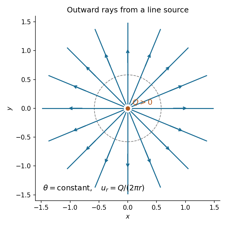
The streamlines are the level curves of the streamfunction, so $\theta$ is constant: radial rays directed outwards from the origin. Their arrows point outwards because $Q>0$. A complete straight line through the origin comprises two distinct rays separated by the excluded line source. Equivalently, $r\dot{\theta }=u_{\theta }=0$ and $\dot{r}=Q/(2\pi r)>0$ along each pathline; the steady flow makes these the same curves as the streamlines.

Set $f(z)=\cosh (\pi z/a)$. The hyperbolic cosine addition formula givesFor $x>0$ and $0<y<a$, both factors in the imaginary part are positive. Thus the image lies in the upper half-plane. The three walls map onto the entire real axis:Also $f^{\prime }(z)=(\pi /a)\sinh (\pi z/a)\ne 0$ in the interior.

To verify that this is a one-to-one conformal map onto the whole upper half-plane, factor it through $s=e^{\pi z/a}$. This first map is one-to-one onto $|s|>1$, $\mathrm{Im}s>0$, and $f(z)=(s+s^{-1})/2$. Given any $\mathrm{Im}\zeta >0$, the roots of $s^2-2\zeta s+1=0$ have product one. Neither lies on $|s|=1$, since that would make $\zeta$ real. Exactly one root therefore has $|s|>1$, andforces that root into the upper half of the exterior disk. It has a unique preimage $z=(a/\pi )(\log |s|+i\arg s)$ with $0<\arg s<\pi$. This proves both surjectivity and injectivity. The construction is the hyperbolic-cosine map of a half-strip.

The source location $c$ is complex, with $\mathrm{Re}c>0$ and $0<\mathrm{Im}c<a$. Put $C=f(c)$, so $\mathrm{Im}C>0$. The method of images places an equal line source at $\bar{C}$ below the real axis:For real $\zeta$, the product of the two logarithm arguments is $|\zeta -C{|}^2>0$. Hence the streamfunction is constant along the wall, on locally consistent branches of the complex logarithm, and there is no normal velocity. Pulling back gives the requested complex potential of a two-dimensional potential flow:This is the line source in a closed-end semi-infinite strip, with no extra imposed flow. Since $f^{\prime }(c)\ne 0$, near the physical source $f(z)-f(c)=f^{\prime }(c)(z-c)+O((z-c{)}^2)$. Thus $w=(Q/(2\pi ))\log (z-c)+$ a regular term, verifying that the source strength remains $Q$ under the conformal map. The image source has no preimage inside the physical strip. Finally, as $x\to \infty$, $w(z)\sim Qz/a+$ a constant, so the far-field velocity is $(Q/a,0)$ and the channel carries exactly the injected volume flux $Q$.

Orient the planar material curve $C(t)$ counterclockwise, and let $\mathbf{t}$ and $\mathbf{n}$ be its unit tangent and outward unit normal vector. The circulation and outward volume flux areFor $\mathbf{u}=(u,v)$ and this orientation, $\mathbf{t}ds=(dx,dy)$ and $\mathbf{n}ds=(dy,-dx)$, givingHere $M$ is the instantaneous flux of the velocity field, rather than transport relative to the moving material curve; that relative transport is zero. If the enclosed region contains no source and the velocity field is smooth there, incompressibility and the planar divergence theorem imply $M=0$.

For smooth inviscid flow of constant mass density under a conservative body force, Kelvin's circulation theorem states that the circulation around any closed material curve is conserved:The constant-mass density assumption is the usual homogeneous incompressible flow setting here. Merely requiring $\nabla \cdot \mathbf{u}=0$ in a fluid of varying mass density would not by itself make the pressure term below a gradient.

Parameterize the material curve by a periodic particle label $s\in [0,1]$, writing ${\mathbf{r}}_t(s,t)=\mathbf{u}(\mathbf{r}(s,t),t)$. Differentiate its line integral, keeping $s$ fixed:The second term vanishes by periodicity. If the conservative body force per unit mass is $-\nabla \Omega$, the Euler momentum equation givesIts line integral around a closed curve is zero, proving the claim. The velocity field must remain smooth on the moving curve, which cannot pass through a line vortex singularity during this argument. No assumption of irrotational flow was needed.

Define the line vortex strength $\kappa$ by $\mathbf{u}=\kappa {\mathbf{e}}_{\theta }/(2\pi r)$, with $\kappa >0$ meaning counterclockwise motion. On an enclosing circle of radius $R$,because the velocity is tangent to the circle. For any simple positively oriented enclosing curve, the same results follow by Stokes theorem and the divergence theorem on the region between that curve and a small inner circle. Both curl and divergence vanish throughout that intervening annulus. ConsequentlyEquivalently, $\Gamma =(\kappa /(2\pi ))\oint d\theta$ and the total angle change is $2\pi$. If strength is instead denoted by $K$ in $u_{\theta }=K/r$, the answer is $\Gamma =2\pi K$. An enclosing disk through the singular origin cannot be used to infer zero circulation from zero local vorticity.

For planar incompressible flow and irrotational flow, combine a velocity potential and a streamfunction into the complex potential of a two-dimensional potential flow:The chosen conventions giveThese are the Cauchy-Riemann equations, so $w$ is a holomorphic function wherever the flow is regular and a consistent local potential is chosen. Its complex derivative is the complex velocityA spatially uniform flow has $w=(U-iV)z+$ a constant. The following contour integral identities also apply to nonuniform potential flow, including the specified line vortex. A complex potential of a two-dimensional potential flow may be multivalued around a source or vortex even though its derivative is single-valued.

Multiply the complex velocity by the complex displacement:The real term is the circulation integrand. With a counterclockwise curve, $\mathbf{n}ds=(dy,-dx)$ is outward, so the imaginary term is the outward volume flux integrand. Integrating givesThis also fixes the sign of $M$: a positive line source has $w^{\prime }=Q/(2\pi z)$ and the integral is $iQ$, so its outward volume flux is $Q$.

Assume $q(z)=w^{\prime }(z)$ is single-valued and a holomorphic function between $C$ and a sufficiently large enclosing circle $|z|=R$. There are no fluid singularities in that region, so Cauchy's integral theorem permits contour deformation:Use the exterior Laurent series about zero, valid for $|z|$ larger than every finite singularity:It converges uniformly on the chosen circle, permitting termwise contour integration. For integer $n$, parameterization by $z=R{e}^{i\theta }$ givesOnly the $z^{-1}$ coefficient survives, provingThus if $b_1=\alpha +i\beta$, then $\Gamma =-2\pi \beta$ and $M=2\pi \alpha$. A uniform flow contributes a constant to $q$ and changes neither integral. The Laurent series here is an exterior expansion; it need not converge in a punctured neighborhood of zero if other singularities intervene.

For the same counterclockwise line vortex strength $\kappa$, its local velocity potential and streamfunction are $\varphi =\kappa \theta /(2\pi )$ and $\psi =-\kappa \log r/(2\pi )$. ConsequentlySubstitution givesin agreement with the direct circulation and volume flux calculation. The sign of the imaginary coefficient is essential for a positive counterclockwise circulation.

Represent a time-harmonic wave by $A\cos (kx-\omega t+\delta )$, with $k,\omega >0$. The angular frequency $\omega$ is the rate at which the wave phase changes at a fixed position, measured in radians per unit time. The wavenumber $k$ is its spatial rate of change, measured in radians per unit length. One full spatial cycle defines the wavelength $\lambda$, and one temporal cycle defines the wave period $T$, soThe ordinary frequency is $f=1/T=\omega /(2\pi )$; the paper's symbol $\omega$ denotes angular frequency.

A fixed wave phase satisfies $kx-\omega t=$ a constant. Differentiating gives the phase velocity, called the wave speed here:It is the speed of an individual crest or other fixed-phase point. The group velocity isevaluated on the relevant dispersion relation. To see its meaning, superpose two equal-amplitude waves with nearby $(k,\omega )$:The slowly varying wave envelope moves with speed $\Delta \omega /\Delta k$, tending to $d\omega /dk$ as the two components approach one another. Thus group velocity describes a narrow wave packet and, for conservative linear surface gravity waves in still water, their energy transport. A single time-harmonic wave has no distinguished packet envelope. When $c=c(k)$, the equivalent relation is $c_g=c+kdc/dk$.

Treat the free surface as the material level set $F(x,y,t)=y-\eta (x,t)=0$. The kinematic boundary condition $DF/Dt=0$, with $\mathbf{u}=\nabla \varphi$, givesThis says that fluid initially on the free surface remains on it.

For constant mass density $\rho$, the Euler momentum equation under gravity is $D\mathbf{u}/Dt=-\nabla p/\rho -g{\mathbf{e}}_y$. Since the flow is irrotational, $(\mathbf{u}\cdot \nabla )\mathbf{u}=\nabla (|\mathbf{u}{|}^2/2)$. Integration in space therefore gives the Unsteady Bernoulli equationAt the free surface, $p=P_a$ and $y=\eta$. Adding a function $G(t)$ to the velocity potential leaves the velocity field unchanged; choose $G^{\prime }=P_a/\rho -B(t)$. With this choice the surface dynamic boundary condition for an inviscid interface becomesThe constant atmospheric pressure has been absorbed into this choice of potential.

Linearize about fluid at rest, with mean free surface $y=0$ and mean bottom $y=-d$. Regard $a$, $\eta$ and the perturbation velocity potential as first-order quantities. A Taylor expansion from $y=\eta$ to $y=0$ produces products of first-order quantities, as do ${\varphi }_x{\eta }_x$ and $|\nabla \varphi {|}^2$. Discarding these second-order terms gives the linearized free-surface boundary conditionsEquivalently, differentiate the second condition in time and substitute the first to obtain ${\varphi }_{tt}+g{\varphi }_y=0$ at $y=0$.

The bottom is also impermeable and moving. Its exact kinematic boundary condition follows from $D(y-h)/Dt=0$:Here $h_t=-akc\cos (k(x-ct))$, while ${\varphi }_x{h}_x$ and the change from evaluating ${\varphi }_y$ at $h$ to evaluating it at $-d$ are second order. HenceThe interior Laplace equation remains ${\varphi }_{xx}+{\varphi }_{yy}=0$ on $-d<y<0$. This linearization requires small slopes and small resulting excursions as well as $a\ll d$; close to resonance a small prescribed bottom displacement can produce a response too large for it.

Seek the periodic response of a surface gravity wave forced by a traveling bottom, with the same wavenumber $k$ and angular frequency $kc$ as the bottom. The linear equations have constant coefficients in $x,t$, so they preserve each such harmonic. There is no dissipative phase lag in this model; away from resonance, the surface response is in phase or in opposition with the bottom. Thus write $\eta =b\sin \theta$, $\theta =k(x-ct)$, with a signed coefficient $b$. Its physical amplitude is $|b|$. Arbitrary additional free surface gravity waves depend on initial data; the paper's expression selects the forced traveling component.

For $k>0$, $c\ne 0$, use $\varphi =F(y)\cos \theta$. The Laplace equation gives $F^{\prime \prime }-k^{2}F=0$. At $y=0$, the two linearized free-surface boundary conditions implyThese determine both constants in the vertical solution:Its vertical derivative at the bottom isMatching it to $-akc\cos \theta$ and multiplying by $c$ givesand thereforeAn equivalent expression for the velocity potential, which makes the bottom condition immediate, isLet ${\omega }_f=kc$ be the forcing angular frequency, and let ${\omega }_0^2=gk\tanh (kd)$ be the natural dispersion relation from Airy wave theory. ThenThe denominator vanishes at $c^2=(g/k)\tanh (kd)$, when the forcing travels at the free-wave phase velocity. For nonzero forcing there is no bounded periodic forced solution at resonance; the undamped linear response develops secular growth. Below that speed $b<0$, giving a phase reversal, while above it $b>0$. At $c=0$ the bottom is stationary: the rest solution has $\varphi =0$ and $\eta =0$, consistent with the zero limit of $b$, though the formula containing $1/c$ must be interpreted through that limit.

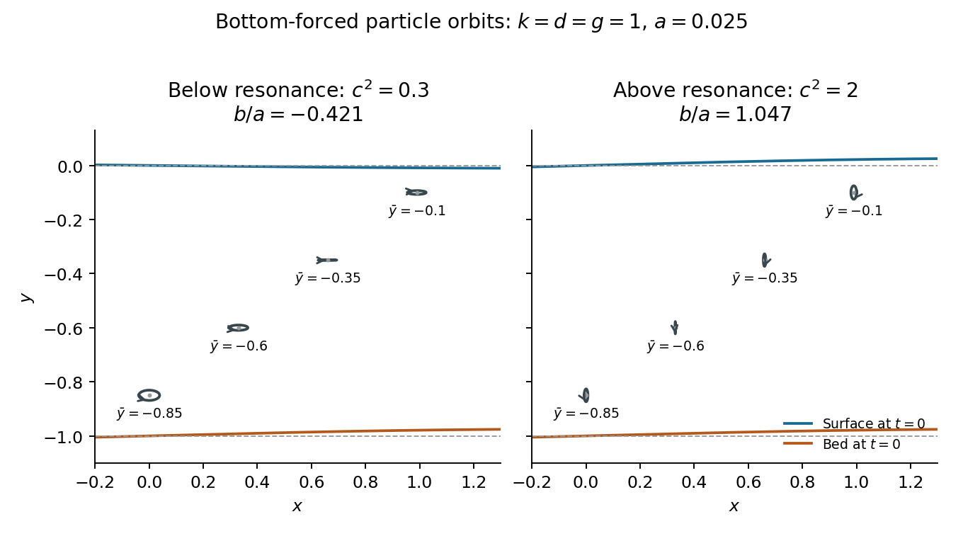
Consider the nonresonant traveling forced solution, with $k>0$ and $c\ne 0$. Put $x=\bar{x}+\xi$, $y=\bar{y}+\upsilon$, where $(\bar{x},\bar{y})$ is the mean position of a fluid element. At linear order, evaluate the velocity field at this mean position: substituting $\xi ,\upsilon$ into its spatial arguments would change the already first-order velocity only at second order. With $\Theta =k(\bar{x}-ct)$, differentiation of the velocity potential givesSince $\dot{\Theta }=-kc$, integration, with zero mean displacements, yieldsIf both coefficients are nonzero, eliminating the wave phase proves that the pathline is an ellipse:Its principal axes of an ellipse are horizontal and vertical, with respective semi-axesThus the full axis lengths are $2|A|$ and $2|B|$. The signed coefficients also determine the direction of traversal. The useful checks $B(0)=b$ and $B(-d)=a$ reproduce the vertical displacements of the free surface and bottom.

To identify the major axis without comparing the two expressions separately, use ${\cosh }^{2}s-{\sinh }^{2}s=1$:Consequently the major axis is horizontal if $c^2<g/k$ and vertical if $c^2>g/k$; equality gives circles. If $A$ or $B$ vanishes at a particular depth, the first-order orbit degenerates to a line segment. These are linearized particle orbits of a bottom-forced gravity wave, not exact closed trajectories at all orders: a higher-order calculation may introduce a mean drift.